Machine learning

class: middle, center

$$ \global\def\myx#1{{\color{green}\mathbf{x}\_{#1}}} $$
$$ \global\def\mys#1{{\color{green}\mathbf{s}\_{#1}}} $$
$$ \global\def\myz#1{{\color{brown}\mathbf{z}\_{#1}}} $$
$$ \global\def\myhnmf#1{{\color{brown}\mathbf{h}\_{#1}}} $$
$$ \global\def\myztilde#1{{\color{brown}\tilde{\mathbf{z}}\_{#1}}} $$
$$ \global\def\myu#1{\mathbf{u}\_{#1}} $$
$$ \global\def\mya#1{\mathbf{a}\_{#1}} $$
$$ \global\def\myv#1{\mathbf{v}\_{#1}} $$
$$ \global\def\mythetaz{\theta\_\myz{}} $$
$$ \global\def\mythetax{\theta\_\myx{}} $$
$$ \global\def\mythetas{\theta\_\mys{}} $$
$$ \global\def\mythetaa{\theta\_\mya{}} $$
$$ \global\def\bs#1{{\boldsymbol{#1}}} $$
$$ \global\def\diag{\text{diag}} $$
$$ \global\def\mbf{\mathbf} $$
$$ \global\def\myh#1{{\color{purple}\mbf{h}\_{#1}}} $$
$$ \global\def\myhfw#1{{\color{purple}\overrightarrow{\mbf{h}}\_{#1}}} $$
$$ \global\def\myhbw#1{{\color{purple}\overleftarrow{\mbf{h}}\_{#1}}} $$
$$ \global\def\myg#1{{\color{purple}\mbf{g}\_{#1}}} $$
$$ \global\def\mygfw#1{{\color{purple}\overrightarrow{\mbf{g}}\_{#1}}} $$
$$ \global\def\mygbw#1{{\color{purple}\overleftarrow{\mbf{g}}\_{#1}}} $$
$$ \global\def\neq{\mathrel{\char`≠}} $$

# Introduction to machine learning

.small-vspace[

]

## Modeling, inference, learning

.vspace[

]

.center[Simon Leglaive]

.vspace[

]

.small.center[CentraleSupélec]

---
class: middle

## Today

The key concepts you should be familiar with at the end of this course are the following:

- **Modeling**, or how to define a model that relates the observed data and the latent variables of interest;
- **Inference**, or how to infer the latent variables from the observations;
- **Learning**, or how to estimate the unkown model parameters from the observed data.

These concepts will be exemplified using the Gaussian mixture model, which will be the focus of the next practical session.

---
class: middle

- The deluge of data calls for automated methods of data analysis, which is what machine learning provides.
  
- Machine learning can be defined as a set of methods that can automatically detect patterns in data, and then use the uncovered patterns to perform predictions and/or make decisions (Murphy, 2012).

- Let's start with an introductory example!

.footnote[Murphy, K. P. (2012). Machine learning: a probabilistic perspective. MIT press.]

---
class: center, middle

.center[ 
  # The adventures of Thomas Bayes, episode 1
]

.block-center-70[
  .medium.center[The following example and drawings are adapted from a [tutorial on Bayesian Learning for Signal Processing](https://members.loria.fr/ADeleforge/files/bayesian_inference_electronic.pdf) given by Antoine Deleforge at the LVA/ICA 2015 Summer School.]
]

---
class: center, middle

![](images/bayes_1.svg)

.left.credit[Image credit: Antoine Deleforge, [Tutorial on Bayesian Learning for Signal Processing](https://members.loria.fr/ADeleforge/files/bayesian_inference_electronic.pdf), LVA/ICA 2015 Summer School]

---
class: center, middle

![](images/bayes_2.svg)

---
class: center, middle

![](images/bayes_3.svg)

---
class: center, middle

![](images/bayes_4.svg)

---
class: center, middle

![](images/bayes_5.svg)

---
class: center, middle

![](images/bayes_6.svg)

---
class: center, middle

![](images/bayes_7.svg)

---
class: center, middle

![](images/bayes_8.svg)

---
class: middle

.grid[

.kol-1-2[

## Data / observations

.width-100[![](images/bayes_data_house.svg)]

]

.kol-1-2[

- The dataset $\mathcal{D}$ consists of $N$ **observations** $\mathbf{x}\_i~\in~\mathbb{R}^D$, $i=1,...,N$.

- Here, $D=2$ and $\mathbf{x}\_i$ corresponds to the coordinates of the $i$-th stone on the ground.

- The observations are assumed to be 
  1. independent and identically distributed (i.i.d);
  2. generated from an unknown probability distribution $p^\star(\mathbf{x})$.

]

.alert[

We write $\mathcal{D} = \left\\{\mathbf{x}\_i~\in~\mathbb{R}^D \overset{i.i.d}{\sim} p^\star(\mathbf{x})\right\\}\_{i=1}^N.$

]

---
class: middle

## Problem

.alert[The problem is to infer a latent variable of interest from the observed data.]
  
Bayes is interested in **inferring** the index of the guilty house, from which the stones were thrown.

This is **the latent variable of interest**, the unkown that we would like to estimate. It is not directly observable, but it is some how **linked** to the observations.

.alert[To solve the problem we need to formalize it.]

To **formalize the problem**, we need to introduce a discrete variable $ z \in \\{1,2,3\\} $ that represents the latent variable and to relate it to the observed data  $\mathcal{D} = \\{\mathbf{x}\_i \in \mathbb{R}^2\\}\_{i=1}^N$ with a **model**. This model defines the link between what is observed and what is unknown.

---
class: middle

## Observation (or likelihood) model

.alert[The observation model explains how the observations are generated from the latent variable.]

Conditionally on $z$, the observations are **assumed** to be i.i.d according to a Gaussian distribution:

$$ p(\mathcal{D} \mid z=k) = p(\mathbf{x}\_1, ..., \mathbf{x}\_N \mid z=k) = \prod\limits\_{i=1}^N p(\mathbf{x}\_i \mid z=k) = \prod\limits\_{i=1}^N \mathcal{N}\left(\mathbf{x}\_i; \boldsymbol{\mu}\_k, \sigma^2\mathbf{I}\right). $$

.grid[

.kol-1-2[

.width-100[![](images/bayes_data_house_likelihood.svg)]

]

.kol-1-2[

- $\\{\boldsymbol{\mu}\_1, \boldsymbol{\mu}\_2, \boldsymbol{\mu}\_3, \sigma^2\\}$ is a set of parameters assumed to be known and fixed;

- $p(\mathcal{D} \mid z=k)$ is the joint distribution of all the observations and it is called the .small[(conditional)] **likelihood**.

.small-vspace[

]

.small[$\mathcal{N}(\mathbf{x}; \boldsymbol{\mu}, \boldsymbol{\Sigma})$ denotes the probability density function (pdf) of the [multivariate Gaussian distribution](https://en.wikipedia.org/wiki/Multivariate_normal_distribution), where $\mathbf{x}$ is the continuous random vector, $\boldsymbol{\mu}$ the mean vector, and $\boldsymbol{\Sigma}$ the covariance matrix.]

]
]

---
class: middle
## Prior model

.alert[The prior model encodes prior information / belief / knowledge about the latent variable of interest.]

Bayes knows that students, grandma Jane and a family with kids live in the first, second and third house, respectively. So he considers the following prior:

.grid[
.kol-1-2[
- $\pi\_1 := p(z = 1) = 0.3$ (student house);
- $\pi\_2 := p(z = 2) = 0.1$ (grandma Jane);
- $\pi\_3 := p(z = 3) = 0.6$ (family with kids).
]
.kol-1-2[
  .right.width-80[![](images/bayes_grandma.svg)]
]
]

.center[What prior could Bayes choose if he did not know the occupants of the different houses?]

.footnote[For the discrete random variable $z$, $p(z = k)$ denotes the probability that it is equal to $k$. $A := B$ reads "A is defined to be B".]

---
class: middle

## Inference

.alert[In the most general case, inference consists in computing or approximating the posterior distribution of the latent variable of interest.

This is achieved by using Bayes' theorem.
]

---

$$
\small{\begin{aligned}
p(z=k \mid \mathcal{D} ) &= \frac{p( \mathcal{D} \mid z=k ) p(z=k)}{ p( \mathcal{D})} & \text{\footnotesize (using Bayes theorem)} \\\\[.65cm]
&= \frac{p( \mathcal{D} \mid z=k ) p(z=k)}{ \sum\limits\_{k=1}^3 p( \mathcal{D}, z=k)} & \text{\footnotesize (using the sum rule)} \\\\[.85cm]
&= \frac{p( \mathcal{D} \mid z=k ) p(z=k)}{ \sum\limits\_{k=1}^3 p( \mathcal{D} \mid z=k) p(z=k)}  & \text{\footnotesize (using the product rule)}\\\\[.65cm]
&= \frac{p(z=k) \prod\limits\_{i=1}^N p( \mathbf{x}\_i \mid z=k )}{ \sum\limits\_{k=1}^3 p(z=k) \prod\limits\_{i=1}^N p( \mathbf{x}\_i \mid z=k ) } & \text{\footnotesize (using the i.i.d assumption)}\\\\[.65cm]
&= \frac{\pi\_k \prod\limits\_{i=1}^N \mathcal{N}\left(\mathbf{x}\_i; \boldsymbol{\mu}\_k, \sigma^2\mathbf{I}\right)}{ \sum\limits\_{k=1}^3 \pi\_k \prod\limits\_{i=1}^N \mathcal{N}\left(\mathbf{x}\_i; \boldsymbol{\mu}\_k, \sigma^2\mathbf{I}\right) } \qquad & \text{\footnotesize (using the prior and observation model)}
\end{aligned}}
$$

???

- Sum rule: $ p(x) = \sum\_y p(x, y) = \sum p(x \mid y) p(y) $

- Product rule: $p(x,y) = p(x\midy) p(y) = p(y\midx) p(x)$

---
class: middle

$$ p(z=k \mid \mathcal{D} ) = \frac{\pi\_k \prod\limits\_{i=1}^N \mathcal{N}\left(\mathbf{x}\_i; \boldsymbol{\mu}\_k, \sigma^2\mathbf{I}\right)}{ \sum\limits\_{k=1}^3 \pi\_k \prod\limits\_{i=1}^N \mathcal{N}\left(\mathbf{x}\_i; \boldsymbol{\mu}\_k, \sigma^2\mathbf{I}\right) }$$

The posterior combines the information from the prior and from the observations. It updates the prior using the observations, through the Bayes' theorem.

We have access to all the quantities necessary to compute the posterior distribution.

.center.width-70[![](images/posterior.svg)]

---
class: middle

## Point estimate

.alert[We are often interested in computing a point estimate of the latent variable of interest from its posterior distribution.]

- The posterior contains all the information about the latent variable we care about, but it does not directly tell Bayes which house is the guilty one.

- From the posterior $ p(z=k \mid \mathcal{D} )$, $k \in \\{1,2,3\\}$, Bayes needs to **make a decision** about the guilty house. 
  
- This is achieved by computing a **point estimate** $\hat{z} \in~\\{1,2,3\\}$, and the posterior probability $p(z=\hat{z} \mid \mathcal{D} )$ indicates how **confident** .small[(or equivalently uncertain)] Bayes is about this decision.

.footnote[In estimation theory and decision theory, the point estimate is called the [Bayes estimator](https://en.wikipedia.org/wiki/Bayes_estimator). It is defined as the minimizer of a posterior expected loss (the expectation of a loss function taken with respect to the posterior distribution). Various loss functions can be defined, leading to different estimates. ]

---
class: middle

A natural choice here is to take the **maximum a posteriori** (MAP) estimate:

$$ \hat{z}\_{\text{MAP}} = \underset{k \in \\{1,2,3\\}}{\arg\max}\, p(z=k \mid \mathcal{D} ) = 1.$$

The students are (estimated) guilty!

.grid[

.kol-3-5[

.center.width-100[![](images/posterior.svg)]

]
.kol-2-5[

.right.width-100[![](images/bayes_pranksters.svg)]

]

---
## Prediction / generation of new data

.alert[We can also predict new data given the already observed ones using the predictive posterior.]

$$\begin{aligned}
p(\mathbf{x}\_{\text{new}} \mid \mathcal{D}) &= \sum\_{k=1}^3 p(\mathbf{x}\_{\text{new}}, z=k \mid \mathcal{D}) & \qquad \text{\footnotesize(using the sum rule)}\\\\
&= \sum\_{k=1}^3 p(\mathbf{x}\_{\text{new}} \mid z=k, \mathcal{D}) p(z=k \mid \mathcal{D}) & \qquad \text{\footnotesize(using the poduct rule)}\\\\
&= \sum\_{k=1}^3 p(\mathbf{x}\_{\text{new}} \mid z=k) p(z=k \mid \mathcal{D}) & \qquad \text{\footnotesize(using the independence assumption)}\\\\
&= \sum\_{k=1}^3 \mathcal{N}(\mathbf{x}\_{\text{new}}; \boldsymbol{\mu}\_k, \sigma^2 \mathbf{I}) p(z=k \mid \mathcal{D}) & \qquad \text{\footnotesize(using the Gaussian observation model)}\\\\
&= \mathbb{E}\_{p(z=k \mid \mathcal{D})}\left[ \mathcal{N}(\mathbf{x}\_{\text{new}}; \boldsymbol{\mu}\_k, \sigma^2 \mathbf{I}) \right] & \qquad \text{\footnotesize(using the definition of the expectation)}
\end{aligned}$$

The predictive posterior is an average of the observation model weighted by the posterior probabilities of $z$.

---
class: middle

The next day, Bayes goes to the university armed with his **predictive posterior**:

.center.width-60[![](images/predictive posterior.svg)]

.center.width-50[![](images/bayes_pred_house.svg)]

---

We can also compute the **predictive prior**, which tells us what we would predict given no observations. This is useful to check if the prior distribution does capture our prior beliefs.

.left-column[

.caption[Predictive prior]
.width-100[![](images/predictive_prior.svg)]

$$ \mathbb{E}\_{p(z=k)}\left[ \mathcal{N}(\mathbf{x}; \boldsymbol{\mu}\_k, \sigma^2 \mathbf{I}) \right] $$

.tiny[1st house: students; 2nd house: grandma; 3rd house: kids]

]

.right-column[

.caption[Predictive posterior]
.width-100[![](images/predictive_posterior_house.svg)]

$$ \mathbb{E}\_{p(z=k \mid \mathcal{D})}\left[ \mathcal{N}(\mathbf{x}; \boldsymbol{\mu}\_k, \sigma^2 \mathbf{I}) \right] $$

]

---
class: middle, center

# Wrap-up 
## Modeling, inference, and learning

---
class: middle

## Starting point

.alert[
We started from the general problem of inferring some latent information from observations in a dataset

$$\mathcal{D} = \left\\{\mathbf{x}\_i \overset{i.i.d}{\sim} p^\star(\mathbf{x})\right\\}\_{i=1}^N.$$
]

---
## Modeling

We formalized the problem by **defining a model that links the observed and the latent variables**.

Following a **generative** approach, this was achieved by defining their **joint distribution**:

$$ p(\mathbf{x}, z ;  \theta) = p(\mathbf{x} \mid z ;  \theta\_x) \, p(z ; \theta\_z), $$

where $\theta = \theta\_x \cup \theta\_z$ and

- $p(\mathbf{x} \mid z ;  \theta\_x)$ is the .small[(conditional)] **likelihood** that defines how observations are generated from the latent variable. It depends on deterministic parameters $\theta\_x$ .small[(mean vectors and variance in Bayes' adventures)];
  - $p(z ; \theta\_z)$ is the **prior** that encodes the prior belief and uncertainty about the latent variable of interest. It depends on deterministic parameters $\theta\_z$ .small[(the prior probabilities in Bayes' adventures)];

.alert[By defining the prior and the likelihood models we are making assumptions about the generative process of the observed data.]

.footnote[

As all observations are assumed to be i.i.d, we drop the index $n$ of $\mathbf{x}\_i$. 
For a discrete (resp. continuous) random variable $z$, $p(z ; \theta\_z)$ denotes its [probability mass function](https://en.wikipedia.org/wiki/Probability_mass_function) (resp. [probability density function](https://en.wikipedia.org/wiki/Probability_density_function)).

]

---
class: middle

By marginalizing the unobserved latent variable in the joint distribution $p(\mathbf{x}, z ;  \theta)$ we obtain the **marginal likelihood**:

$$
p(\mathbf{x}; \theta) = \begin{cases}
\displaystyle\int\_\mathcal{Z} p(\mathbf{x} \mid z; \theta\_x)\, p(z; \theta\_z) dz \qquad \text{\footnotesize if $z \in \mathcal{Z}$ is continuous}; \\\\[.5cm]
\displaystyle\sum\limits\_{k \in \mathcal{Z}} p(\mathbf{x} \mid z = k ; \theta\_x)\, p(z = k; \theta\_z) \qquad \text{\footnotesize if $z \in \mathcal{Z}$ is discrete}.
\end{cases} 
$$

.alert[The marginal likelihood $p(\mathbf{x}; \theta)$ is a model of the distribution $p^\star(\mathbf{x})$ that is assumed to have generated the observations in the dataset.
]

---
class: middle

## Inference

.alert[Inference consists in computing the posterior distribution of the latent variable, which summarizes our knowledge on $z$ once we have observed $\mathbf{x}$.]

- Using **Bayes' theorem**, the posterior distribution writes:
  $$p(z \mid \mathbf{x}; \theta) = \frac{p(\mathbf{x}\mid z; \theta\_x) p(\mathbf{z} ; \theta\_z) }{ p(\mathbf{x}; \theta)}.$$

- The process of inference will often require us to use the posterior to answer various questions.

---
## Point estimate

- $p(z \mid \mathbf{x}; \theta)$ encodes all our knowledge about $z$ after observing the data, but it does not directly provide an "estimate" of the $z$. From the posterior, we need to choose a single value $\hat{z}$ to serve as a **point estimate** of $z$.  In Bayesian statistics, this is a **decision**, and in different contexts we might want to select different point estimates.

- To take the decision, we need to introduce a **loss function** $\mathcal{l}(\hat{z}, z)$ which tells us "how bad" would $\hat{z}$ be if the "true value" of the latent variable was $z$. The decision is then taken by minimizing the **posterior expected loss**:

$$ \mathcal{L}(\hat{z}) = \mathbb{E}\_{p(z \mid \mathbf{x}; \theta)}[\mathcal{l}(\hat{z}, z)].$$

- For example, if we consider a continuous latent variable and the squared error loss ${\ell(\hat{z}, z) = (\hat{z} - z)^2}$, we obtain the **posterior mean** estimate:

$$ \hat{z}\_{MSE} =  \underset{\hat{z}}{\arg\min}\,  \mathbb{E}\_{p(z \mid \mathbf{x}; \theta)}[(\hat{z} - z)^2] = \mathbb{E}\_{p(z \mid \mathbf{x}; \theta)}[z ].$$

---
## Uncertainty

- Importantly, the posterior distribution encodes **uncertainty** about the latent variable of interest. Indeed, we inferred a full probability distribution and did not simply compute a point estimate.

- Quantifying uncertaining when making predictions is important for critical applications such as in medicine, autonomous driving, etc.

- Uncertainty can be quantified using a [credible interval](https://easystats.github.io/bayestestR/articles/credible_interval.html#:~:text=As%20the%20Bayesian%20inference%20returns,contains%2095%25%20of%20the%20values.), which is just an interval within which the latent variable value falls with a particular probability.

.left-column[

.center.width-80[![](images/credible_interval.png)]

]

.right-column[

$[a, b]$ is the 95% credible interval for the continuous latent variable $z$ if

$$ \int_{a}^b p(z \mid \mathbf{x}; \theta) dz = 0.95.$$

]

.reset-column[

]

.credit[Image credits: [bayestestR](https://easystats.github.io/bayestestR/articles/credible_interval.html#:~:text=As%20the%20Bayesian%20inference%20returns,contains%2095%25%20of%20the%20values)]

---
class: middle 
## Prediction / generation of new data

- **Predictive prior**

"Averaging" the likelihood over the prior:

$$\begin{aligned}
  p(\mathbf{x}\_{\text{new}}; \theta) &= \mathbb{E}\_{p(z ; \theta\_z)}[p(\mathbf{x}\_{\text{new}} \mid z ; \theta\_x )].
  \end{aligned}$$

- **Predictive posterior**

"Averaging" the likelihood over the posterior:

$$\begin{aligned}
  p(\mathbf{x}\_{\text{new}} \mid \mathbf{x} ; \theta) &= \mathbb{E}\_{p(z \mid \mathbf{x} ; \theta)}[p(\mathbf{x}\_{\text{new}} \mid z  ; \theta\_x )].
  \end{aligned}$$

---
class: middle, center

## Wait, what about **learning**, as in machine **learning**?

---
class: middle

## Learning

In the adventures of Thomas Bayes, we ended-up with the following decision rule:

$$ \hat{z} = \underset{k \in \\{1,2,3\\}}{\arg\max}\, p(z=k \mid \mathcal{D} ; \theta ) =  \underset{k \in \\{1,2,3\\}}{\arg\max}\,  \frac{\pi\_k \prod\limits\_{i=1}^N \mathcal{N}\left(\mathbf{x}\_i; \boldsymbol{\mu}\_k, \sigma^2\mathbf{I}\right)}{ \sum\limits\_{k=1}^3 \pi\_k \prod\limits\_{i=1}^N \mathcal{N}\left(\mathbf{x}\_i; \boldsymbol{\mu}\_k, \sigma^2\mathbf{I}\right) }$$

This is a function of:

- the input **data** in $\mathcal{D} = \left\\{\mathbf{x}\_i \overset{i.i.d}{\sim} p^\star(\mathbf{x})\right\\}\_{i=1}^N$;
- the **model parameters** $\theta = \left\\{ \sigma^2, \left\\{\boldsymbol{\mu}\_k, \pi\_k\right\\}_{k=1}^3 \right\\}$, which were assumed to be known and fixed.

.alert[Learning is the process to automatically estimate the model parameters from the data.]

---
class: middle

.alert[Many models in machine learning can be studied from a probabilistic perspective, where learning consists in estimating the parameters $\theta$ that make the .bold[model] distribution $p(\mathbf{x} ; \theta)$ as close as possible to the true data distribution $p^\star(\mathbf{x})$, given a .bold[dataset] of i.i.d observations and a .bold[measure of fit].]

.left-column[
The three main ingredients to formalize learning in probabilistic machine learing are 
- A model distribution $p(\mathbf{x} ; \theta)$, which may or may not involve latent variables; 
- A dataset $\mathcal{D} = \left\\{\mathbf{x}\_i \overset{i.i.d}{\sim} p^\star(\mathbf{x})\right\\}\_{i=1}^N$; 
- A measure of fit between $p(\mathbf{x} ; \theta)$ and $p^\star(\mathbf{x})$, seen as a function of $\theta$.
]
.right-column[
.width-100[![](images/distrib_fitting.png)]
]

---
class: middle

## KL divergence and maximum likelihood

- A popular choice is to take the Kullback-Leibler (KL) divergence as a measure of fit:

$$D\_{\text{KL}}(p \parallel q) = \mathbb{E}\_{p}[ \ln(p) - \ln(q)] \ge 0,$$

with equality if and only if $p=q$ and $D\_{\text{KL}}(p \parallel q) \neq D\_{\text{KL}}(q \parallel p)$.

- Then **learning consists in solving the following optimization problem**:

$$ 
  \begin{aligned}
  & \underset{\theta}{\min}\hspace{.1cm} \Bigg\\{ D\_{\text{KL}} (p^\star(\mathbf{x}) \parallel p(\mathbf{x}; \theta))  =  \mathbb{E}\_{p^\star(\mathbf{x})}[ \ln p^\star(\mathbf{x}) - \ln p(\mathbf{x}; \theta)] \Bigg\\} 
  \Leftrightarrow \underset{\theta}{\max}\hspace{.1cm} \mathbb{E}\_{p^\star(\mathbf{x})}[ \ln p(\mathbf{x}; \theta)].
  \end{aligned}
  $$
  
- The difficulty is that we do not know the true data distribution $p^\star(\mathbf{x})$, which prevents us from computing the expectation analytically.

---
class: middle

- We use the **Monte Carlo method**, which approximates the intractable expectation by an empirical average using i.i.d samples drawn from $p^\star(\mathbf{x})$:

$$ \mathbb{E}\_{p^\star(\mathbf{x})} [ \ln p(\mathbf{x}; \theta) ] \approx \frac{1}{N}  \sum\_{i=1}^N \ln p(\mathbf{x}\_i; \theta).$$

- This last expression shows that **choosing the Kullback-Leibler divergence as the measure of fit leads to maximum (log-marginal) likelihood parameters estimation**.

We are trying to find the model parameters that are the most likely on average over the dataset, where "being likely" means that the corresponding log-density $\ln p(\mathbf{x}; \theta)$ is high whhen evaluated on the samples of the dataset.

.footnote[The Monte Carlo estimator is unbiased and converges almost surely towards the exact expectation as the number of samples tends to infinity.]

---
class: middle, center

Which distribution better fits the data?

.center.width-90[![](images/illust_Gaussian.svg)]

---
class: middle

## Summary

.alert-g.left[

- **Data**: Get the dataset $\mathcal{D} = \left\\{\mathbf{x}\_i \overset{i.i.d}{\sim} p^\star(\mathbf{x})\right\\}\_{i=1}^N$.
- **Modeling**: Define a model that relates the latent variable of interest to the observations $p(\mathbf{x},z; \theta) = p(\mathbf{x} \mid z; \theta\_x) p(z; \theta\_z)$.
- **Inference**: Compute the posterior distribution $p(z \mid \mathbf{x} ; \theta)$, which can then be used in many different ways.
- **Learning**: Estimate the unknown model parameters $\theta$ by maximizing the log-marginal likelihood $\ln p(\mathbf{x}; \theta)$ averaged over the dataset.

]

.footnote[
When the observations or the latent variables are natural signals or images, we are actually doing signal processing using ML.
]

---
exclude: true
class: middle, center

# Taking a step back and looking at the landscape of machine learning

---
exclude: true
class: middle

What we have seen so far actually corresponds to a subset of machine learning methods, involving
- **generative modeling**, because we define a generative model of the observed data; 
- **Bayesian modeling and inference**, because the generative model involves a latent random variable equiped with a prior and during inference we compute its posterior distribution;
- **unsupervised learning**, because the parameters of the model, which .italic[in fine] allow us to infer the latent variable of interest from the observations through the posterior, are learned from unlabeled data.

.alert-g[**Supervised learning** is another important subset of machine learning methods, which involves generative or **discriminative models**. This will be the topic of another lecture.]

---
exclude: true
class: middle

- Supervised learning with discriminative models is probably the dominating paradigm in machine learning, which has led to great research and industrial successes in recent years.

- But understanding first unsupervised learning with generative models greatly helps to have a deep understanding of supervised learning with discriminative models.

- This is for three reasons:

1. The whole story of extracting a latent variable of interest from observations is always valid **at test time**, whatever the machine learning method.
  2. Supervised learning is simply the case where, **at training time**, the variable of interest is not latent anymore but observed and used for the learning of the model parameters (no need to marginalize it anymore!);
  3. Discriminative modeling is simply the case where we directly define the posterior distribution in the modeling step, instead of defining the joint distribution and then using Bayes theorem.

---
exclude: true
class: middle

.center.width-90[![](images/unsupervised_supervised_ML.svg)]

.credit[Credits: [Antoine Deleforge](https://members.loria.fr/ADeleforge/lectures/), Inria, course given at Télécom Physique Strasbourg.]

---
exclude: true
class: middle
## Applications of unsupervised learning

.center.width-80[![](images/applications_unsupervised_learning.svg)]

.alert[Potential to learn from massive amount of unlabeled data to generate even more.]

.credit[Credits: [Antoine Deleforge](https://members.loria.fr/ADeleforge/lectures/), Inria, course given at Télécom Physique Strasbourg.]

---
exclude: true
class: middle
## Fundamental techniques in unsupervised learning

.center.width-80[![](images/fundamentals_unsupervised_learning.svg)]

These fundamental techniques can all be described from a probabilistic perspective, where 
- the structure of the latent variable of interest $z$ is encoded in a suitable probabilistic prior (**modeling**); 
- the task of extracting $z$ from the observations corresponds to the computation of its posterior (**inference**); 
- the model parameters are estimated by maximizing the marginal likelihood (**learning**).

.credit[Image credits: [Antoine Deleforge](https://members.loria.fr/ADeleforge/lectures/), Inria, course given at Télécom Physique Strasbourg.]

---
exclude: true
class: middle

## Machine learning for signal processing

.alert[When the observations or the latent variables correspond to natural signals or images, we are actually doing signal processing using machine learning.]

---
exclude: true
class: middle

The previous fundamental techniques form the basis of many advanced deep learning techniques used today:

- Variational autoencoders (VAEs);
- Generative adversarial networks (GANs);
- Normalizing flow;
- Diffusion models;
- Conditional neural processes;
- Self-supervised learning;
- etc.

---
class: middle

In the adventures of Thomas Bayes, episode 1, we discovered the modeling and inference steps, but not the learning step (the model parameters were assumed to be known and fixed).

---
class: center, middle

.center[ 
  # The adventures of Thomas Bayes, episode 2
]

---
class: center, middle

![](images/bayes1.svg)

---
class: center, middle

![](images/bayes2.svg)

---
class: center, middle

![](images/bayes3.svg)

---
class: center, middle

![](images/bayes4.svg)

---
class: middle, center
### Modeling

---

.left-column[

**Observed variables**: $ \\{\mathbf{x}\_i \in \mathbb{R}^2\\}\_{i=1}^N$.

.width-80.center[![](images/bayes_observations.svg)]

** Generative model **

.width-40.center[![](images/BN_example.svg)]

$$ p(\\{\mathbf{x}\_i, z\_i\\}\_{i=1}^N; \theta) = \prod\limits\_{i=1}^N p(\mathbf{x}\_i , z\_i; \theta) = \prod\limits\_{i=1}^N p(\mathbf{x}\_i \mid z\_i; \theta) p(z\_i; \theta). $$

]

.right-column[

**Hidden variables**: $ \\{z\_i \in \\{1,2,3\\} \\}\_{i=1}^N$.

.width-90.center[![](images/bayes_latents_1.svg)]

]

---

.grid[

.kol-1-2[

.vspace[
    
  ]
  .width-50.center[![](images/BN_example.svg)]

]

.kol-1-2[

.width-70.center[![](images/bayes_latents_1.svg)]
  
]

.kol-1-4[
**Prior**
]
.kol-3-4[
$ p(z\_i = k; \theta) = \pi\_k, \qquad  \sum\limits\_{k=1}^K \pi\_k = 1, \qquad K=3$ 
]

.kol-1-4[
**Likelihood**
]
.kol-3-4[
$ p(\mathbf{x}\_i \mid z\_i=k ; \theta) = \mathcal{N}\left(\mathbf{x}\_i; \boldsymbol{\mu}\_k, \boldsymbol{\Sigma}\_k \right)$
]

.kol-1-4[
**Parameters**
]
.kol-3-4[
$\theta = \\{\pi\_k, \boldsymbol{\mu}\_k, \boldsymbol{\Sigma}\_k \\}\_{k=1}^K.$ 
]

]
---

**Marginal likelihood**

$$
\begin{aligned}
p(\\{\mathbf{x}\_i\\}\_{i=1}^N; \theta) &= \prod\_{i=1}^N p(\mathbf{x}\_i ; \theta) \\\\
&= \prod\_{i=1}^N \sum\_{k=1}^{K} p(\mathbf{x}\_i \mid z\_i = k ; \theta) p(z\_i = k; \theta)  \\\\
&= \prod\_{i=1}^N \sum\_{k=1}^{K} \pi\_k \mathcal{N}\left(\mathbf{x}\_i; \boldsymbol{\mu}\_k, \boldsymbol{\Sigma}\_k \right).
\end{aligned}
$$

Observations are independent and identically distributed according to a **Gaussian mixture model** (GMM) with $K=3$ components.

The parameters $\pi\_k$ are called the **mixing coefficients**, they give the prior probability of picking the k-th component to generate a data point $\mathbf{x}\_i$.

???

$$
\begin{aligned}
p(\mathbf{x}\_1, \mathbf{x}\_2) &= \sum\_{j, k} p(\mathbf{x}\_1, \mathbf{x}\_2, z\_1=j, z\_2=k) \\\\
&= \sum\_{j, k} p(\mathbf{x}\_1\mid z\_1=j) p(z\_1=j) p(\mathbf{x}\_2 \mid z\_2=k) p(z\_2=k) \\\\
&= \sum\_{j} \left[ \sum\_{k} p(\mathbf{x}\_1\mid z\_1=j) p(z\_1=j) p(\mathbf{x}\_2 \mid z\_2=k) p(z\_2=k) \right] \\\\
&= \sum\_{j} p(\mathbf{x}\_1\mid z\_1=j) p(z\_1=j) \left[ \sum\_{k}  p(\mathbf{x}\_2 \mid z\_2=k) p(z\_2=k) \right] \\\\
&= p(\mathbf{x}\_1) p(\mathbf{x}\_2) \\\\
\end{aligned}
$$

---
class: middle, center
### Inference

---

**Posterior distribution**

.grid[

.kol-1-2[

$ p\left(\\{z\_i\\}\_{i=1}^N \mid \\{\mathbf{x}\_i\\}\_{i=1}^N; \theta\right) = \prod\limits\_{i=1}^N p(z\_i \mid \mathbf{x}\_i; \theta), $

where

$
\begin{aligned}
p(z\_i = k \mid \mathbf{x}\_i; \theta) &= \frac{ p(\mathbf{x}\_i \mid z\_i = k; \theta) p(z\_i = k; \theta) }{p(\mathbf{x}\_i ; \theta)} \\\\[.3cm]
&= \frac{ p(\mathbf{x}\_i \mid z\_i = k; \theta) p(z\_i = k; \theta) }{\sum\_{j=1}^K p(\mathbf{x}\_i \mid z\_i = j; \theta) p(z\_i = j; \theta)  } \\\\[.5cm]
&= \frac{ \pi\_k p(\mathbf{x}\_i \mid z\_i = k; \theta) }{\sum\_{j=1}^K \pi\_j p(\mathbf{x}\_i \mid z\_i = j; \theta)  }.
\end{aligned}
$

]

.kol-1-2[

.width-90.right[![](images/bayes_latents_2.svg)]  
]

]

The posterior probabilities $p(z\_i = k \mid \mathbf{x}\_i; \theta)$ are also known as the **responsabilities**.

The argmax of the responsability assigns the observation to a component, i.e. it **clusters the data**.

---

**Parameters estimation**

The posterior distribution can be computed analytically, but it depends on the **unknown model parameters** $\theta = \\{\pi\_k, \boldsymbol{\mu}\_k, \boldsymbol{\Sigma}\_k \\}\_{k=1}^K$.

Ideally, we would like to estimate them by maximizing the log-marginal likelihood:

$$ 
\begin{aligned}
\mathcal{L}(\theta) &= \ln p(\\{\mathbf{x}\_i\\}\_{i=1}^N; \theta) \\\\
&= \ln \prod\_{i=1}^N \sum\_{k=1}^{K} \pi\_k \mathcal{N}\left(\mathbf{x}\_i; \boldsymbol{\mu}\_k, \boldsymbol{\Sigma}\_k \right) \\\\
&= \sum\_{i=1}^N \ln \left(\sum\_{k=1}^{K} \pi\_k \mathcal{N}\left(\mathbf{x}\_i; \boldsymbol{\mu}\_k, \boldsymbol{\Sigma}\_k \right) \right).
\end{aligned}$$

Due to the presence of the sum over $k$ inside the logarithm, **the maximum marginal likelihood solution for the parameters does not have a closed-form analytical solution.**

---
count: false
class: center, middle

.width-90.center[![](images/bayes_EM.svg)]

---
class: center, middle

## The expectation-maximization algorithm

---
class: middle

The expectation-maximization (EM) algorithm is a general technique introduced by Dempster et al. in 1977 for maximum likelihood parameters estimation in probabilistic models having latent variables.

Let $\mathbf{x} \in \mathcal{X}$ and $\mathbf{z} \in \mathcal{Z}$ denote the **observed and latent** random variables, respectively, which are assumed to be continuous, although the discussion is identical in the discrete setting.

We assume that direct optimization of the marginal likelihood $p(\mathbf{x}; {\theta})$ is difficult, while optimization of the complete-data likelihood function $p(\mathbf{x}, \mathbf{z} ; \theta)$ is much simpler.

---
### The evidence lower bound

We first introduce a distribution over the latent variables whose probability density function is denoted by $q(\mathbf{z})$.

For any distribution $q(\mathbf{z})$, the following decomposition of the log-marginal likelihood holds:

$$ \ln p(\mathbf{x}; \theta) = \mathcal{L}(q(\mathbf{z}), \theta) + D\_{\text{KL}}(q(\mathbf{z} ) \parallel p(\mathbf{z} \mid \mathbf{x}; \theta)),$$

where $\mathcal{L}(q(\mathbf{z}), \theta)$ is called the **evidence lower bound** (ELBO), and it is defined by

$$ \mathcal{L}(q(\mathbf{z}), \theta) = \mathbb{E}\_{q(\mathbf{z})} [\ln p(\mathbf{x}, \mathbf{z}; \theta) - \ln q(\mathbf{z} )]. $$

The **Kullback-Leibler** (KL) divergence is defined by:

$$D\_{\text{KL}}(q \parallel p) = \mathbb{E}\_{q}[ \ln(q) - \ln(p)],$$

and it satisfies $D\_{\text{KL}}(q \parallel p) \ge 0$ with equality if and only if $q = p$.

--- 
.small[Proof:] $\scriptsize \ln p(\mathbf{x}; \theta) = \mathbb{E}\_{q(\mathbf{z})}[\ln p(\mathbf{x}; \theta)] = \mathbb{E}\_{q(\mathbf{z})}[\ln p(\mathbf{x}, \mathbf{z}; \theta) - \ln p(\mathbf{z} \mid \mathbf{x}; \theta) - \ln q(\mathbf{z}) + \ln q(\mathbf{z}) ] $

---

$$ \ln p(\mathbf{x}; \theta) = \mathcal{L}(q(\mathbf{z}), \theta) + D\_{\text{KL}}(q(\mathbf{z} ) \parallel p(\mathbf{z} \mid \mathbf{x}; \theta))$$

<hr>

As the KL divergence is always non-negative, we have:

$$\ln p(\mathbf{x}; \theta) \ge \mathcal{L}(q(\mathbf{z}), \theta), $$

with equality if and only if $q(\mathbf{z}) = p(\mathbf{z} \mid \mathbf{x}; \theta)$.

The ELBO is indeed a **lower bound of the log-marginal likelihood**, which is tight if $q(\mathbf{z})$ matches the true posterior.

.width-40.center[![](images/ELBO-bishop.png)]

.credit[Image credit: Christopher M. Bishop, [Pattern Recognition and Machine Learning](https://www.microsoft.com/en-us/research/uploads/prod/2006/01/Bishop-Pattern-Recognition-and-Machine-Learning-2006.pdf), Springer, 2006.]

---
### EM algorithm

The EM algorithm is an iterative algorithm which alternates between optimizing the ELBO with respect to $q$ in the E-Step and with repspect to $\theta$ in the M-step.

We first **initialize** $\theta\_0$, then we iterate for $t \ge 0$

- **E-Step**: $ q\_{t+1}(\mathbf{z}) = \underset{q}{\arg\max}\, \mathcal{L}(q(\mathbf{z}), \theta\_{t})  $

- **M-Step**: $ \theta\_{t+1} = \underset{\theta}{\arg\max}\, \mathcal{L}(q\_{t+1}(\mathbf{z}), \theta)  $

---
### E-Step

We recall the decomposition of the log-marginal likelihood:

$$ \ln p(\mathbf{x}; \theta) = \mathcal{L}(q(\mathbf{z}), \theta) + D\_{\text{KL}}(q(\mathbf{z} ) \parallel p(\mathbf{z} \mid \mathbf{x}; \theta)).$$

The solution of the E-step is given by:

$$
  \begin{aligned}
  q\_{t+1}(\mathbf{z}) &= \underset{q}{\arg\max}\, \mathcal{L}(q(\mathbf{z}), \theta\_{t}) \\\\[.5cm]
  &= \underset{q}{\arg\min}\, D\_{\text{KL}}(q(\mathbf{z} ) \parallel p(\mathbf{z} \mid \mathbf{x}; \theta\_{t})) \\\\[.5cm]
  &= p(\mathbf{z} \mid \mathbf{x}; \theta\_{t}).
  \end{aligned}
  $$

---

class: middle

After the E-Step, we have $D\_{\text{KL}}(q\_{t+1}(\mathbf{z} ) \parallel p(\mathbf{z} \mid \mathbf{x}; \theta\_{t})) = 0$, and the ELBO is equal to the log-marginal likelihood (i.e. the lower-bound is tight):

$$ \ln p(\mathbf{x}; \theta\_t) = \mathcal{L}(q\_{t+1}(\mathbf{z}), \theta\_t). $$

.small-vspace[

]

.width-50.center[![](images/ELBO-bishop-2.png)]

Therefore, maximizing the lower-bound with respect to the model parameters in the M-step will necessarily increase the log-marginal likelihood.

---
### M-Step

- We recall the expression of the ELBO:

$$ \mathcal{L}(q(\mathbf{z}), \theta) = \mathbb{E}\_{q(\mathbf{z})} [\ln p(\mathbf{x}, \mathbf{z}; \theta) - \ln q(\mathbf{z} )], $$

- The solution of the M-step is given by:

$$
  \begin{aligned}
  \theta\_{t+1} &= \underset{\theta}{\arg\max}\, \mathcal{L}(q\_{t+1}(\mathbf{z}), \theta) \\\\[.5cm]
   &= \underset{\theta}{\arg\max}\, \mathcal{L}\big( p(\mathbf{z} \mid \mathbf{x}; \theta\_{t}), \theta\big) \\\\[.5cm]
   &= \underset{\theta}{\arg\max}\, \mathbb{E}\_{ p(\mathbf{z} \mid \mathbf{x}; \theta\_{t})} [\ln p(\mathbf{x}, \mathbf{z}; \theta) - \ln  p(\mathbf{z} \mid \mathbf{x}; \theta\_{t})] \\\\[.5cm]
   &= \underset{\theta}{\arg\max}\, \mathbb{E}\_{ p(\mathbf{z} \mid \mathbf{x}; \theta\_{t})} [\ln p(\mathbf{x}, \mathbf{z}; \theta) ] + cst(\theta),
  \end{aligned}
  $$

where the constant is the differential entropy of $p(\mathbf{z} \mid \mathbf{x}; \theta\_{t})$ which is independent of $\theta$.

---

.footnote[We recall the decomposition of the log-marginal likelihood $ \ln p(\mathbf{x}; \theta) = \mathcal{L}(q(\mathbf{z}), \theta) + D\_{\text{KL}}(q(\mathbf{z} ) \parallel p(\mathbf{z} \mid \mathbf{x}; \theta)).$]

After the M-step, because $q\_{t+1}(\mathbf{z} ) = p(\mathbf{z} \mid \mathbf{x}; \theta\_{t})$ has been held fixed for computing the new model parameters $\theta\_{t+1}$, the KL divergence $D\_{\text{KL}}(q\_{t+1}(\mathbf{z} ) \parallel p(\mathbf{z} \mid \mathbf{x}; \theta\_{t+1}))$ will be non zero.

The increase in the log-marginal likelihood function is therefore greater than the increase in the ELBO, as shown below.

.width-40.center[![](images/ELBO-bishop-3.png)]

---

.grid[

.kol-1-3[
  Initialize $\theta\_0$.
]
.kol-2-3[
.width-90.right[![](images/MM0.png)]
]

]

---
count: false

.grid[

.kol-1-3[
Iteration $t=1$:

- **E-Step**:

$\qquad q\_{1}(\mathbf{z}) = p(\mathbf{z} \mid \mathbf{x}; \theta\_0)$

]
.kol-2-3[
.width-90.right[![](images/MM1.png)]
]

]

We have $D\_{\text{KL}}(q\_{1}(\mathbf{z}) \parallel p(\mathbf{z} \mid \mathbf{x}; \theta\_{0})) = 0 $ such that $\ln p(\mathbf{x}; \theta\_0) = \mathcal{L}(q\_{1}(\mathbf{z}), \theta\_0)$.

---
count: false

.grid[

.kol-1-3[
Iteration $t=1$:

- E-Step:

$\qquad q\_{1}(\mathbf{z}) = p(\mathbf{z} \mid \mathbf{x}; \theta\_0)$

- **M-Step**:

$\theta\_1 = \underset{\theta}{\arg\max}\, \mathcal{L}(q\_{1}(\mathbf{z}), \theta)  $

]
.kol-2-3[
.width-90.right[![](images/MM2.png)]
]

]

---
count: false

.grid[

.kol-1-3[
Iteration $t=1$:

- E-Step:

$\qquad q\_{1}(\mathbf{z}) = p(\mathbf{z} \mid \mathbf{x}; \theta\_0)$

- M-Step:

$\theta\_1 = \underset{\theta}{\arg\max}\, \mathcal{L}(q\_{1}(\mathbf{z}), \theta)  $

]
.kol-2-3[
.width-90.right[![](images/MM3.png)]
]

]

We have $D\_{\text{KL}}(q\_{1}(\mathbf{z} ) \parallel p(\mathbf{z} \mid \mathbf{x}; \theta\_{1})) \neq 0$.

---
count: false

.grid[

.kol-1-3[
Iteration $t=2$:

- **E-Step**:

$\qquad q\_{2}(\mathbf{z}) = p(\mathbf{z} \mid \mathbf{x}; \theta\_1)$

]
.kol-2-3[
.width-90.right[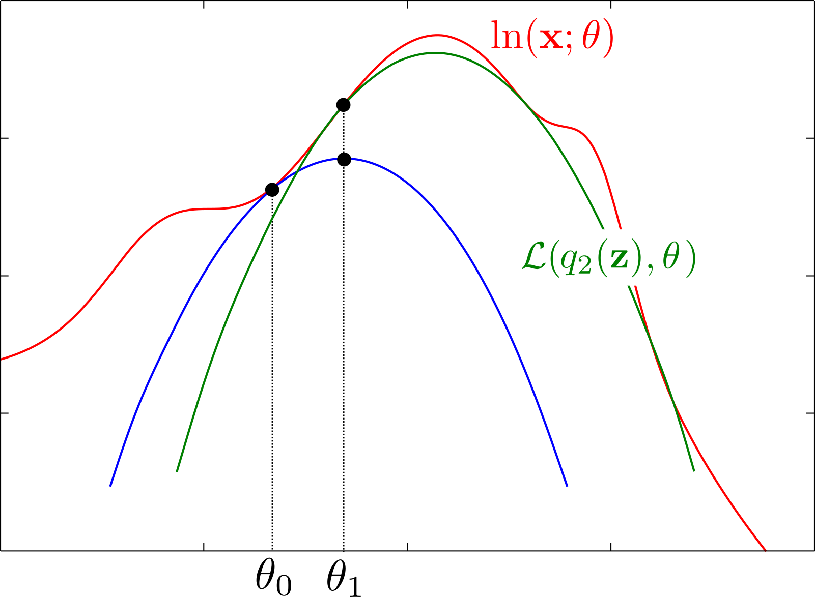![](images/MM4.png)]
]

]

We have $D\_{\text{KL}}(q\_{2}(\mathbf{z}) \parallel p(\mathbf{z} \mid \mathbf{x}; \theta\_{1})) = 0 $ such that $\ln p(\mathbf{x}; \theta\_1) = \mathcal{L}(q\_{2}(\mathbf{z}), \theta\_1)$.

---
count: false

.grid[

.kol-1-3[
Iteration $t=2$:

- E-Step:

$\qquad q\_{2}(\mathbf{z}) = p(\mathbf{z} \mid \mathbf{x}; \theta\_1)$

- **M-Step**:

$\theta\_2 = \underset{\theta}{\arg\max}\, \mathcal{L}(q\_{2}(\mathbf{z}), \theta)  $

]
.kol-2-3[
.width-90.right[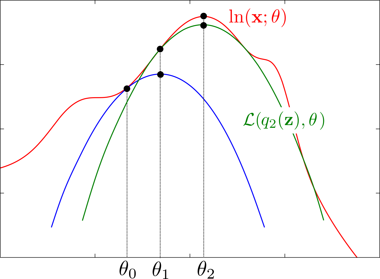![](images/MM5.png)]
]

]

---
count: false

.grid[

.kol-1-3[
Iteration $t=2$:

- E-Step:

$\qquad q\_{2}(\mathbf{z}) = p(\mathbf{z} \mid \mathbf{x}; \theta\_1)$

- M-Step:

$\theta\_2 = \underset{\theta}{\arg\max}\, \mathcal{L}(q\_{2}(\mathbf{z}), \theta)  $

- **We reached a stationary point.**

]
.kol-2-3[
.width-90.right[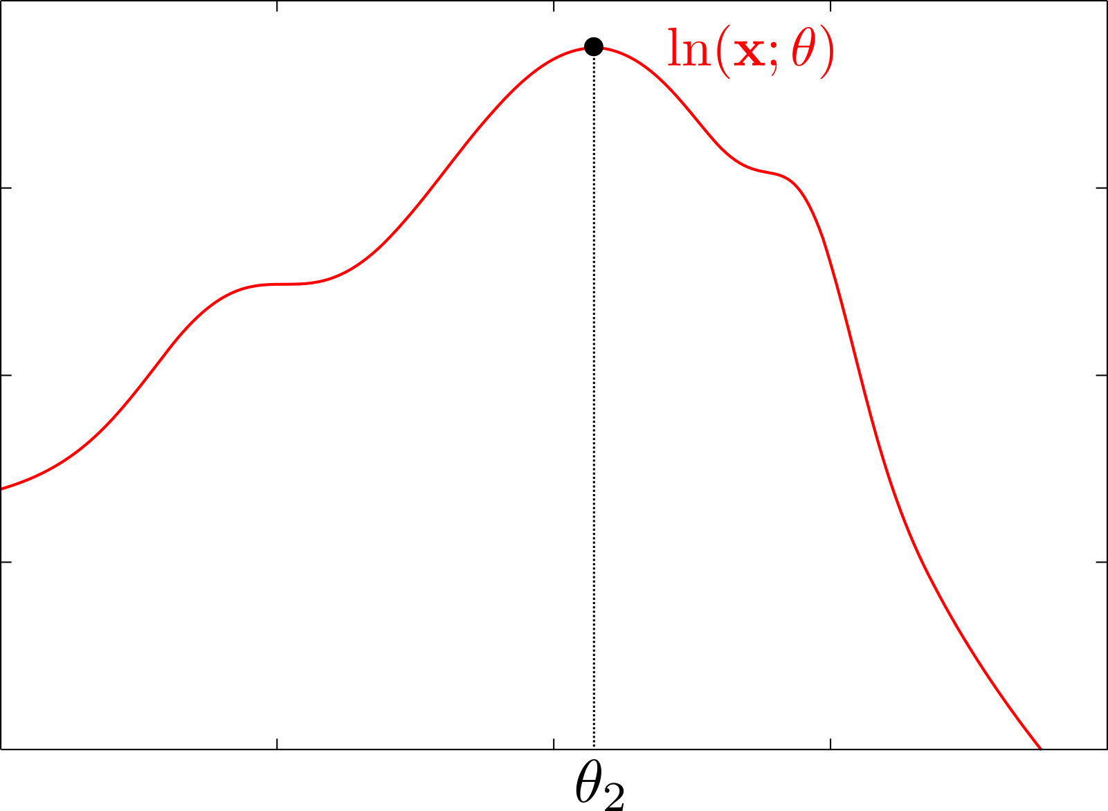![](images/MM6.png)]
]

]

---
### Properties of the EM algorithm

- The log-marginal likelihood is **monotonically increasing**.

--
count: false

--- 
.bold[Proof]:

Using the fact that $ \ln p(\mathbf{x}; \theta) = \mathcal{L}(q(\mathbf{z}), \theta) + D\_{\text{KL}}(q(\mathbf{z} ) \parallel p(\mathbf{z} \mid \mathbf{x}; \theta))$ and $q\_{t+1}(\mathbf{z}) = p(\mathbf{z} \mid \mathbf{x}; \theta\_{t})$ we deduce:

$$\mathcal{L}(q\_{t+1}(\mathbf{z}), \theta\_{t}) = \ln p(\mathbf{x}; \theta\_{t}),$$

$$\mathcal{L}(q\_{t+1}(\mathbf{z}), \theta\_{t+1}) \le \ln p(\mathbf{x}; \theta\_{t+1}). $$

Moreover, by definintion of the M-step:

$$\mathcal{L}(q\_{t+1}(\mathbf{z}), \theta\_{t+1}) \ge \mathcal{L}(q\_{t+1}(\mathbf{z}), \theta\_{t}). $$

Putting all together we have:

$$ \ln p(\mathbf{x}; \theta\_{t+1}) \ge \mathcal{L}(q\_{t+1}(\mathbf{z}), \theta\_{t+1}) \ge \mathcal{L}(q\_{t+1}(\mathbf{z}), \theta\_{t}) = \ln p(\mathbf{x}; \theta\_{t}). $$

---

---
count: false

### Properties of the EM algorithm

- The log-marginal likelihood is **monotonically increasing**.
- The algorithm converges to a **stationary point** of the log-marginal likelihood.
- As the problem is generally not convex, the algorithm generally converges to a local optimum which strongly **depends on the initialization**.

---
### EM algorithm summary

The EM algorithm can be reformulated in the space of the model parameters only.

Given an initialization $\theta\_0$ of the model parameters, iterate for $t=0:T-1$:

- **E-Step**: $Q(\theta, \theta\_t) = \mathbb{E}\_{ p(\mathbf{z} \mid \mathbf{x}; \theta\_{t})} [\ln p(\mathbf{x}, \mathbf{z}; \theta) ]$;

- **M-Step**: $\theta\_{t+1} = \underset{\theta}{\arg\max}\, Q(\theta, \theta\_t) $.

.bold[This is the recipe you should remember and use to derive an EM algorithm.]

---
## Back to the adventures of Thomas Bayes

.width-90.center[![](images/bayes_EM.svg)]

---
class: middle

.grid[

.kol-1-2[

![](images/EM-GMM1.svg)

]

.kol-1-2[

- Initialization: Random "guess" for $\theta\_0$
- E-Step: $Q(\theta, \theta\_t) = \mathbb{E}\_{ p(\mathbf{z} \mid \mathbf{x}; \theta\_{t})} [\ln p(\mathbf{x}, \mathbf{z}; \theta) ]$
- M-Step: $\theta\_{t+1} = \arg\max\_\theta\, Q(\theta, \theta\_t) $
- Convergence

]

---
class: middle
count: false

.grid[

.kol-1-2[

![](images/EM-GMM2.svg)

]

.kol-1-2[

- **Initialization**: Random "guess" for $\theta\_0$
- E-Step: $Q(\theta, \theta\_t) = \mathbb{E}\_{ p(\mathbf{z} \mid \mathbf{x}; \theta\_{t})} [\ln p(\mathbf{x}, \mathbf{z}; \theta) ]$
- M-Step: $\theta\_{t+1} = \arg\max\_\theta\, Q(\theta, \theta\_t) $
- Convergence

]
]

---
class: middle
count: false

.grid[

.kol-1-2[

![](images/EM-GMM3.svg)

]

.kol-1-2[

- Initialization: Random "guess" for $\theta\_0$
- **E-Step**: $Q(\theta, \theta\_t) = \mathbb{E}\_{ p(\mathbf{z} \mid \mathbf{x}; \theta\_{t})} [\ln p(\mathbf{x}, \mathbf{z}; \theta) ]$
- M-Step: $\theta\_{t+1} = \arg\max\_\theta\, Q(\theta, \theta\_t) $
- Convergence

]
]

---
class: middle
count: false

.grid[

.kol-1-2[

![](images/EM-GMM4.svg)

]

.kol-1-2[

- Initialization: Random "guess" for $\theta\_0$
- E-Step: $Q(\theta, \theta\_t) = \mathbb{E}\_{ p(\mathbf{z} \mid \mathbf{x}; \theta\_{t})} [\ln p(\mathbf{x}, \mathbf{z}; \theta) ]$
- **M-Step**: $\theta\_{t+1} = \arg\max\_\theta\, Q(\theta, \theta\_t) $
- Convergence

]
]

---
class: middle
count: false

.grid[

.kol-1-2[

![](images/EM-GMM5.svg)

]

.kol-1-2[

]
]

---
class: middle
count: false

.grid[

.kol-1-2[

![](images/EM-GMM6.svg)

]

.kol-1-2[

- Initialization: Random "guess" for $\theta\_0$
- E-Step: $Q(\theta, \theta\_t) = \mathbb{E}\_{ p(\mathbf{z} \mid \mathbf{x}; \theta\_{t})} [\ln p(\mathbf{x}, \mathbf{z}; \theta) ]$
- **M-Step**: $\theta\_{t+1} = \arg\max\_\theta\, Q(\theta, \theta\_t) $
- Convergence

]
]

---
class: middle
count: false

.grid[

.kol-1-2[

![](images/EM-GMM7.svg)

]

.kol-1-2[

]
]

---
class: middle
count: false

.grid[

.kol-1-2[

![](images/EM-GMM8.svg)

]

.kol-1-2[

- Initialization: Random "guess" for $\theta\_0$
- E-Step: $Q(\theta, \theta\_t) = \mathbb{E}\_{ p(\mathbf{z} \mid \mathbf{x}; \theta\_{t})} [\ln p(\mathbf{x}, \mathbf{z}; \theta) ]$
- **M-Step**: $\theta\_{t+1} = \arg\max\_\theta\, Q(\theta, \theta\_t) $
- Convergence

]
]

---
class: middle
count: false

.grid[

.kol-1-2[

![](images/EM-GMM9.svg)

]

.kol-1-2[

]
]

---
class: middle
count: false

.grid[

.kol-1-2[

![](images/EM-GMM10.svg)

]

.kol-1-2[

- Initialization: Random "guess" for $\theta\_0$
- E-Step: $Q(\theta, \theta\_t) = \mathbb{E}\_{ p(\mathbf{z} \mid \mathbf{x}; \theta\_{t})} [\ln p(\mathbf{x}, \mathbf{z}; \theta) ]$
- **M-Step**: $\theta\_{t+1} = \arg\max\_\theta\, Q(\theta, \theta\_t) $
- Convergence

]
]

---
class: middle
count: false

.grid[

.kol-1-2[

![](images/EM-GMM11.svg)

]

.kol-1-2[

]
]

---
class: middle
count: false

.grid[

.kol-1-2[

![](images/EM-GMM12.svg)

]

.kol-1-2[

]
]

---
class: middle, center

.grid[

.kol-1-2[

![](images/EM-GMM12.svg)

]

.kol-1-2[

.big-vspace[

]

.width-80.center[![](images/bayes_EM_2.svg)]

]
]

---
class: middle

## Lab session

- Theoretical work: Derivation of the EM algorithm for the GMM model.
- Practical work: Implementation of the EM algorithm.