Bayesian Methods for Machine Learning

class: middle, center

$$ \global\def\myx#1{{\color{green}\mathbf{x}\_{#1}}} $$
$$ \global\def\mys#1{{\color{green}\mathbf{s}\_{#1}}} $$
$$ \global\def\myz#1{{\color{brown}\mathbf{z}\_{#1}}} $$
$$ \global\def\myhnmf#1{{\color{brown}\mathbf{h}\_{#1}}} $$
$$ \global\def\myztilde#1{{\color{brown}\tilde{\mathbf{z}}\_{#1}}} $$
$$ \global\def\myu#1{\mathbf{u}\_{#1}} $$
$$ \global\def\mya#1{\mathbf{a}\_{#1}} $$
$$ \global\def\myv#1{\mathbf{v}\_{#1}} $$
$$ \global\def\mythetaz{\theta\_\myz{}} $$
$$ \global\def\mythetax{\theta\_\myx{}} $$
$$ \global\def\mythetas{\theta\_\mys{}} $$
$$ \global\def\mythetaa{\theta\_\mya{}} $$
$$ \global\def\bs#1{{\boldsymbol{#1}}} $$
$$ \global\def\diag{\text{diag}} $$
$$ \global\def\mbf{\mathbf} $$
$$ \global\def\myh#1{{\color{purple}\mbf{h}\_{#1}}} $$
$$ \global\def\myhfw#1{{\color{purple}\overrightarrow{\mbf{h}}\_{#1}}} $$
$$ \global\def\myhbw#1{{\color{purple}\overleftarrow{\mbf{h}}\_{#1}}} $$
$$ \global\def\myg#1{{\color{purple}\mbf{g}\_{#1}}} $$
$$ \global\def\mygfw#1{{\color{purple}\overrightarrow{\mbf{g}}\_{#1}}} $$
$$ \global\def\mygbw#1{{\color{purple}\overleftarrow{\mbf{g}}\_{#1}}} $$

# Bayesian Methods for Machine Learning

.small-vspace[

]

### Lecture 1 - Fundamentals of Bayesian modeling and inference

.bold[Simon Leglaive]

.tiny[CentraleSupélec]

---
class: middle

## Today

The key concepts you should be familiar with at the end of this course are the following:

- **Modeling** (how to define a Bayesian model);
- **Inference** (how to perform inference);
- **Learning** (how to learn the parameters of a model).

---
class: middle

- The deluge of data calls for automated methods of data analysis, which is what machine learning provides.
  
- Machine learning can be defined as a set of methods that can automatically detect patterns in data, and then use the uncovered patterns to perform predictions and/or make decisions (Murphy, 2012).

- Let's start with an introductory example!

.footnote[Murphy, K. P. (2012). Machine learning: a probabilistic perspective. MIT press.]

---
class: center, middle

.center[ 
  # The adventures of Thomas Bayes, episode 1
]

.block-center-70[
  .medium.center[The following example and drawings are adapted from a [tutorial on Bayesian Learning for Signal Processing](https://members.loria.fr/ADeleforge/files/bayesian_inference_electronic.pdf) given by Antoine Deleforge at the LVA/ICA 2015 Summer School.]
]

---
class: center, middle

![](images/bayes_1.svg)

.left.credit[Image credit: Antoine Deleforge, [Tutorial on Bayesian Learning for Signal Processing](https://members.loria.fr/ADeleforge/files/bayesian_inference_electronic.pdf), LVA/ICA 2015 Summer School]

---
class: center, middle

![](images/bayes_2.svg)

---
class: center, middle

![](images/bayes_3.svg)

---
class: center, middle

![](images/bayes_4.svg)

---
class: center, middle

![](images/bayes_5.svg)

---
class: center, middle

![](images/bayes_6.svg)

---
class: center, middle

![](images/bayes_7.svg)

---
class: center, middle

![](images/bayes_8.svg)

---
class: middle

.grid[

.kol-1-2[

## Data / observations

.width-100[![](images/bayes_data_house.svg)]

]

.kol-1-2[

- The dataset $\mathcal{D}$ consists of $N$ **observations** $\mathbf{x}\_i~\in~\mathbb{R}^D$, $i=1,...,N$.

- Here, $D=2$ and $\mathbf{x}\_i$ corresponds to the coordinates of the $i$-th stone on the ground.

- The observations are assumed to be 
  1. independent and identically distributed (i.i.d);
  2. generated from an unknown probability distribution $p^\star(\mathbf{x})$.

]

.alert[

We write $\mathcal{D} = \left\\{\mathbf{x}\_i~\in~\mathbb{R}^D \overset{i.i.d}{\sim} p^\star(\mathbf{x})\right\\}\_{i=1}^N.$

]

---
class: middle

## Problem

.alert[The problem is to infer a latent variable of interest from the observed data.]
  
Bayes is interested in **inferring** the index of the guilty house, from which the stones were thrown.

This is **the latent variable of interest**, the unkown that we would like to estimate. It is not directly observable, but it is some how **linked** to the observations.

.alert[To solve the problem we need to formalize it.]

To **formalize the problem**, we need to introduce a discrete variable $ z \in \\{1,2,3\\} $ that represents the latent variable and to relate it to the observed data  $\mathcal{D} = \\{\mathbf{x}\_i \in \mathbb{R}^2\\}\_{i=1}^N$ with a **model**. This model defines the link between what is observed and what is unknown.

---
class: middle

## Observation (or likelihood) model

.alert[The observation model explains how the observations are generated from the latent variable.]

Conditionally on $z$, the observations are **assumed** to be i.i.d according to a Gaussian distribution:

$$ p(\mathcal{D} \mid z=k) = p(\mathbf{x}\_1, ..., \mathbf{x}\_N \mid z=k) = \prod\limits\_{i=1}^N p(\mathbf{x}\_i \mid z=k) = \prod\limits\_{i=1}^N \mathcal{N}\left(\mathbf{x}\_i; \boldsymbol{\mu}\_k, \sigma^2\mathbf{I}\right). $$

.grid[

.kol-1-2[

.width-100[![](images/bayes_data_house_likelihood.svg)]

]

.kol-1-2[

- $\\{\boldsymbol{\mu}\_1, \boldsymbol{\mu}\_2, \boldsymbol{\mu}\_3, \sigma^2\\}$ is a set of parameters assumed to be known and fixed;

- $p(\mathcal{D} \mid z=k)$ is the joint distribution of all the observations and it is called the .small[(conditional)] **likelihood**.

.small-vspace[

]

.small[$\mathcal{N}(\mathbf{x}; \boldsymbol{\mu}, \boldsymbol{\Sigma})$ denotes the probability density function (pdf) of the [multivariate Gaussian distribution](https://en.wikipedia.org/wiki/Multivariate_normal_distribution), where $\mathbf{x}$ is the continuous random vector, $\boldsymbol{\mu}$ the mean vector, and $\boldsymbol{\Sigma}$ the covariance matrix.]

]
]

---
class: middle
## Prior model

.alert[The prior model encodes prior information / belief / knowledge about the latent variable of interest.]

Bayes knows that students, grandma Jane and a family with kids live in the first, second and third house, respectively. So he considers the following prior:

.grid[
.kol-1-2[
- $\pi\_1 := p(z = 1) = 0.3$ (student house);
- $\pi\_2 := p(z = 2) = 0.1$ (grandma Jane);
- $\pi\_3 := p(z = 3) = 0.6$ (family with kids).
]
.kol-1-2[
  .right.width-80[![](images/bayes_grandma.svg)]
]
]

.center[What prior could Bayes choose if he did not know the occupants of the different houses?]

.footnote[For the discrete random variable $z$, $p(z = k)$ denotes the probability that it is equal to $k$. $A := B$ reads "A is defined to be B".]

---
class: middle

## Inference

.alert[In the most general case, inference consists in computing or approximating the posterior distribution of the latent variable of interest.

This is achieved by using Bayes' theorem.
]

---

$$
\small{\begin{aligned}
p(z=k \mid \mathcal{D} ) &= \frac{p( \mathcal{D} \mid z=k ) p(z=k)}{ p( \mathcal{D})} & \text{\footnotesize (using Bayes theorem)} \\\\[.65cm]
&= \frac{p( \mathcal{D} \mid z=k ) p(z=k)}{ \sum\limits\_{j=1}^3 p( \mathcal{D}, z=j)} & \text{\footnotesize (using the sum rule)} \\\\[.85cm]
&= \frac{p( \mathcal{D} \mid z=k ) p(z=k)}{ \sum\limits\_{j=1}^3 p( \mathcal{D} \mid z=j) p(z=j)}  & \text{\footnotesize (using the product rule)}\\\\[.65cm]
&= \frac{p(z=k) \prod\limits\_{i=1}^N p( \mathbf{x}\_i \mid z=k )}{ \sum\limits\_{j=1}^3 p(z=j) \prod\limits\_{i=1}^N p( \mathbf{x}\_i \mid z=j ) } & \text{\footnotesize (using the i.i.d assumption)}\\\\[.65cm]
&= \frac{\pi\_k \prod\limits\_{i=1}^N \mathcal{N}\left(\mathbf{x}\_i; \boldsymbol{\mu}\_k, \sigma^2\mathbf{I}\right)}{ \sum\limits\_{j=1}^3 \pi\_j \prod\limits\_{i=1}^N \mathcal{N}\left(\mathbf{x}\_i; \boldsymbol{\mu}\_j, \sigma^2\mathbf{I}\right) } \qquad & \text{\footnotesize (using the prior and observation model)}
\end{aligned}}
$$

???

- Sum rule: $ p(x) = \sum\_y p(x, y) = \sum p(x | y) p(y) $

- Product rule: $p(x,y) = p(x|y) p(y) = p(y|x) p(x)$

---
class: middle

$$ p(z=k \mid \mathcal{D} ) = \frac{\pi\_k \prod\limits\_{i=1}^N \mathcal{N}\left(\mathbf{x}\_i; \boldsymbol{\mu}\_k, \sigma^2\mathbf{I}\right)}{ \sum\limits\_{j=1}^3 \pi\_j \prod\limits\_{i=1}^N \mathcal{N}\left(\mathbf{x}\_i; \boldsymbol{\mu}\_j, \sigma^2\mathbf{I}\right) }$$

The posterior combines the information from the prior and from the observations. It updates the prior using the observations, through the Bayes' theorem.

We have access to all the quantities necessary to compute the posterior distribution.

.center.width-70[![](images/posterior.svg)]

---
class: middle

## Point estimate

.alert[We are often interested in computing a point estimate of the latent variable of interest from its posterior distribution.]

- The posterior contains all the information about the latent variable we care about, but it does not directly tell Bayes which house is the guilty one.

- From the posterior $ p(z=k \mid \mathcal{D} )$, $k \in \\{1,2,3\\}$, Bayes needs to **make a decision** about the guilty house. 
  
- This is achieved by computing a **point estimate** $\hat{z} \in~\\{1,2,3\\}$, and the posterior probability $p(z=\hat{z} \mid \mathcal{D} )$ indicates how **confident** .small[(or equivalently uncertain)] Bayes is about this decision.

.footnote[In estimation theory and decision theory, the point estimate is called the [Bayes estimator](https://en.wikipedia.org/wiki/Bayes_estimator). It is defined as the minimizer of a posterior expected loss (the expectation of a loss function taken with respect to the posterior distribution). Various loss functions can be defined, leading to different estimates. ]

---
class: middle

A natural choice here is to take the **maximum a posteriori** (MAP) estimate:

$$ \hat{z}\_{\text{MAP}} = \underset{k \in \\{1,2,3\\}}{\arg\max}\, p(z=k \mid \mathcal{D} ) = 1.$$

The students are (estimated) guilty!

.grid[

.kol-3-5[

.center.width-100[![](images/posterior.svg)]

]
.kol-2-5[

.right.width-100[![](images/bayes_pranksters.svg)]

]

---
## Prediction / generation of new data

.alert[We can also predict new data given the already observed ones using the predictive posterior.]

$$\begin{aligned}
p(\mathbf{x}\_{\text{new}} \mid \mathcal{D}) &= \sum\_{k=1}^3 p(\mathbf{x}\_{\text{new}}, z=k \mid \mathcal{D}) & \qquad \text{\footnotesize(using the sum rule)}\\\\
&= \sum\_{k=1}^3 p(\mathbf{x}\_{\text{new}} \mid z=k, \mathcal{D}) p(z=k \mid \mathcal{D}) & \qquad \text{\footnotesize(using the poduct rule)}\\\\
&= \sum\_{k=1}^3 p(\mathbf{x}\_{\text{new}} \mid z=k) p(z=k \mid \mathcal{D}) & \qquad \text{\footnotesize(using the independence assumption)}\\\\
&= \sum\_{k=1}^3 \mathcal{N}(\mathbf{x}\_{\text{new}}; \boldsymbol{\mu}\_k, \sigma^2 \mathbf{I}) p(z=k \mid \mathcal{D}) & \qquad \text{\footnotesize(using the Gaussian observation model)}\\\\
&= \mathbb{E}\_{p(z=k \mid \mathcal{D})}\left[ \mathcal{N}(\mathbf{x}\_{\text{new}}; \boldsymbol{\mu}\_k, \sigma^2 \mathbf{I}) \right] & \qquad \text{\footnotesize(using the definition of the expectation)}
\end{aligned}$$

The predictive posterior is an average of the observation model weighted by the posterior probabilities of $z$.

---
class: middle

The next day, Bayes goes to the university armed with his **predictive posterior**:

.center.width-60[![](images/predictive posterior.svg)]

.center.width-50[![](images/bayes_pred_house.svg)]

---

We can also compute the **predictive prior**, which tells us what we would predict given no observations. This is useful to check if the prior distribution does capture our prior beliefs.

.left-column[

.caption[Predictive prior]
.width-100[![](images/predictive_prior.svg)]

$$ \mathbb{E}\_{p(z=k)}\left[ \mathcal{N}(\mathbf{x}; \boldsymbol{\mu}\_k, \sigma^2 \mathbf{I}) \right] $$

.tiny[1st house: students; 2nd house: grandma; 3rd house: kids]

]

.right-column[

.caption[Predictive posterior]
.width-100[![](images/predictive_posterior_house.svg)]

$$ \mathbb{E}\_{p(z=k \mid \mathcal{D})}\left[ \mathcal{N}(\mathbf{x}; \boldsymbol{\mu}\_k, \sigma^2 \mathbf{I}) \right] $$

]

---
class: middle, center

# Wrap-up 
## Modeling, inference, and learning

---
class: middle

## Starting point

.alert[
We started from the general problem of inferring some latent information from observations in a dataset

$$\mathcal{D} = \left\\{\mathbf{x}\_i \overset{i.i.d}{\sim} p^\star(\mathbf{x})\right\\}\_{i=1}^N.$$
]

---
## Modeling

We formalized the problem by **defining a model that links the observed and the latent variables**.

Following a **generative** approach, this was achieved by defining their **joint distribution**:

$$ p(\mathbf{x}, z ;  \theta) = p(\mathbf{x} \mid z ;  \theta\_x) \, p(z ; \theta\_z), $$

where $\theta = \theta\_x \cup \theta\_z$ and

- $p(\mathbf{x} \mid z ;  \theta\_x)$ is the .small[(conditional)] **likelihood** that defines how observations are generated from the latent variable. It depends on deterministic parameters $\theta\_x$ .small[(mean vectors and variance in Bayes' adventures)];
  - $p(z ; \theta\_z)$ is the **prior** that encodes the prior belief and uncertainty about the latent variable of interest. It depends on deterministic parameters $\theta\_z$ .small[(the prior probabilities in Bayes' adventures)];

.alert[By defining the prior and the likelihood models we are making assumptions about the generative process of the observed data.]

.footnote[

As all observations are assumed to be i.i.d, we drop the index $n$ of $\mathbf{x}\_i$. 
For a discrete (resp. continuous) random variable $z$, $p(z ; \theta\_z)$ denotes its [probability mass function](https://en.wikipedia.org/wiki/Probability_mass_function) (resp. [probability density function](https://en.wikipedia.org/wiki/Probability_density_function)).

]

---
class: middle

By marginalizing the unobserved latent variable in the joint distribution $p(\mathbf{x}, z ;  \theta)$ we obtain the **marginal likelihood**:

$$
p(\mathbf{x}; \theta) = \begin{cases}
\displaystyle\int\_\mathcal{Z} p(\mathbf{x} \mid z; \theta\_x)\, p(z; \theta\_z) dz \qquad \text{\footnotesize if $z \in \mathcal{Z}$ is continuous}; \\\\[.5cm]
\displaystyle\sum\limits\_{k \in \mathcal{Z}} p(\mathbf{x} \mid z = k ; \theta\_x)\, p(z = k; \theta\_z) \qquad \text{\footnotesize if $z \in \mathcal{Z}$ is discrete}.
\end{cases} 
$$

.alert[The marginal likelihood $p(\mathbf{x}; \theta)$ is a model of the distribution $p^\star(\mathbf{x})$ that is assumed to have generated the observations in the dataset.
]

---
class: middle

## Inference

.alert[Inference consists in computing the posterior distribution of the latent variable, which summarizes our knowledge on $z$ once we have observed $\mathbf{x}$.]

- Using **Bayes' theorem**, the posterior distribution writes:
  $$p(z \mid \mathbf{x}; \theta) = \frac{p(\mathbf{x}\mid z; \theta\_x) p(z ; \theta\_z) }{ p(\mathbf{x}; \theta)}.$$

- The process of inference will often require us to use the posterior to answer various questions.

---
## Point estimate

- $p(z \mid \mathbf{x}; \theta)$ encodes all our knowledge about $z$ after observing the data, but it does not directly provide an "estimate" of the $z$. From the posterior, we need to choose a single value $\hat{z}$ to serve as a **point estimate** of $z$.  In Bayesian statistics, this is a **decision**, and in different contexts we might want to select different point estimates.

- To take the decision, we need to introduce a **loss function** $\mathcal{l}(\hat{z}, z)$ which tells us "how bad" would $\hat{z}$ be if the "true value" of the latent variable was $z$. The decision is then taken by minimizing the **posterior expected loss**:

$$ \mathcal{L}(\hat{z}) = \mathbb{E}\_{p(z \mid \mathbf{x}; \theta)}[\mathcal{l}(\hat{z}, z)].$$

- For example, if we consider a continuous latent variable and the squared error loss ${\ell(\hat{z}, z) = (\hat{z} - z)^2}$, we obtain the **posterior mean** estimate:

$$ \hat{z}\_{MSE} =  \underset{\hat{z}}{\arg\min}\,  \mathbb{E}\_{p(z \mid \mathbf{x}; \theta)}[(\hat{z} - z)^2] = \mathbb{E}\_{p(z \mid \mathbf{x}; \theta)}[z ].$$

---
## Uncertainty

- Importantly, the posterior distribution encodes **uncertainty** about the latent variable of interest. Indeed, we inferred a full probability distribution and did not simply compute a point estimate.

- Quantifying uncertaining when making predictions is important for critical applications such as in medicine, autonomous driving, etc.

- Uncertainty can be quantified using a [credible interval](https://easystats.github.io/bayestestR/articles/credible_interval.html#:~:text=As%20the%20Bayesian%20inference%20returns,contains%2095%25%20of%20the%20values.), which is just an interval within which the latent variable value falls with a particular probability.

.left-column[

.center.width-80[![](images/credible_interval.png)]

]

.right-column[

$[a, b]$ is the 95% credible interval for the continuous latent variable $z$ if

$$ \int_{a}^b p(z \mid \mathbf{x}; \theta) dz = 0.95.$$

]

.reset-column[

]

.credit[Image credits: [bayestestR](https://easystats.github.io/bayestestR/articles/credible_interval.html#:~:text=As%20the%20Bayesian%20inference%20returns,contains%2095%25%20of%20the%20values)]

---
class: middle 
## Prediction / generation of new data

- **Predictive prior**

"Averaging" the likelihood over the prior:

$$\begin{aligned}
  p(\mathbf{x}\_{\text{new}}; \theta) &= \mathbb{E}\_{p(z ; \theta\_z)}[p(\mathbf{x}\_{\text{new}} \mid z ; \theta\_x )].
  \end{aligned}$$

- **Predictive posterior**

"Averaging" the likelihood over the posterior:

$$\begin{aligned}
  p(\mathbf{x}\_{\text{new}} \mid \mathbf{x} ; \theta) &= \mathbb{E}\_{p(z \mid \mathbf{x} ; \theta)}[p(\mathbf{x}\_{\text{new}} \mid z  ; \theta\_x )].
  \end{aligned}$$

---
class: middle, center

## Wait, what about **learning**, as in machine **learning**?

---
class: middle

## Learning

In the adventures of Thomas Bayes, we ended-up with the following decision rule:

$$ \hat{z} = \underset{k \in \\{1,2,3\\}}{\arg\max}\, p(z=k \mid \mathcal{D} ; \theta ) =  \underset{k \in \\{1,2,3\\}}{\arg\max}\,  \frac{\pi\_k \prod\limits\_{i=1}^N \mathcal{N}\left(\mathbf{x}\_i; \boldsymbol{\mu}\_k, \sigma^2\mathbf{I}\right)}{ \sum\limits\_{j=1}^3 \pi\_j \prod\limits\_{i=1}^N \mathcal{N}\left(\mathbf{x}\_i; \boldsymbol{\mu}\_j, \sigma^2\mathbf{I}\right) }$$

This is a function of:

- the input **data** in $\mathcal{D} = \left\\{\mathbf{x}\_i \overset{i.i.d}{\sim} p^\star(\mathbf{x})\right\\}\_{i=1}^N$;
- the **model parameters** $\theta = \left\\{ \sigma^2, \left\\{\boldsymbol{\mu}\_k, \pi\_k\right\\}_{k=1}^3 \right\\}$, which were assumed to be known and fixed.

.alert[Learning is the process to automatically estimate the model parameters from the data.]

---
class: middle

.alert[Many models in machine learning can be studied from a probabilistic perspective, where learning consists in estimating the parameters $\theta$ that make the .bold[model] distribution $p(\mathbf{x} ; \theta)$ as close as possible to the true data distribution $p^\star(\mathbf{x})$, given a .bold[dataset] of i.i.d observations and a .bold[measure of fit].]

.left-column[
The three main ingredients to formalize learning in probabilistic machine learing are 
- A model distribution $p(\mathbf{x} ; \theta)$, which may or may not involve latent variables; 
- A dataset $\mathcal{D} = \left\\{\mathbf{x}\_i \overset{i.i.d}{\sim} p^\star(\mathbf{x})\right\\}\_{i=1}^N$; 
- A measure of fit between $p(\mathbf{x} ; \theta)$ and $p^\star(\mathbf{x})$, seen as a function of $\theta$.
]
.right-column[
.width-100[![](images/distrib_fitting.png)]
]

---
class: middle

## KL divergence and maximum likelihood

- A popular choice is to take the Kullback-Leibler (KL) divergence as a measure of fit:

$$D\_{\text{KL}}(p \parallel q) = \mathbb{E}\_{p}[ \ln(p) - \ln(q)] \ge 0,$$

with equality if and only if $p=q$ and $D\_{\text{KL}}(p \parallel q) \neq D\_{\text{KL}}(q \parallel p)$.

- Then **learning consists in solving the following optimization problem**:

$$ 
  \begin{aligned}
  & \underset{\theta}{\min}\hspace{.1cm} \Bigg\\{ D\_{\text{KL}} (p^\star(\mathbf{x}) \parallel p(\mathbf{x}; \theta))  =  \mathbb{E}\_{p^\star(\mathbf{x})}[ \ln p^\star(\mathbf{x}) - \ln p(\mathbf{x}; \theta)] \Bigg\\} 
  \Leftrightarrow \underset{\theta}{\max}\hspace{.1cm} \mathbb{E}\_{p^\star(\mathbf{x})}[ \ln p(\mathbf{x}; \theta)].
  \end{aligned}
  $$
  
- The difficulty is that we do not know the true data distribution $p^\star(\mathbf{x})$, which prevents us from computing the expectation analytically.

---
class: middle

- We use the **Monte Carlo method**, which approximates the intractable expectation by an empirical average using i.i.d samples drawn from $p^\star(\mathbf{x})$:

$$ \mathbb{E}\_{p^\star(\mathbf{x})} [ \ln p(\mathbf{x}; \theta) ] \approx \frac{1}{N}  \sum\_{i=1}^N \ln p(\mathbf{x}\_i; \theta).$$

- This last expression shows that **choosing the Kullback-Leibler divergence as the measure of fit leads to maximum (log-marginal) likelihood parameters estimation**.

We are trying to find the model parameters that are the most likely on average over the dataset, where "being likely" means that the corresponding log-density $\ln p(\mathbf{x}; \theta)$ is high when evaluated on the samples of the dataset.

.footnote[The Monte Carlo estimator is unbiased and converges almost surely towards the exact expectation as the number of samples tends to infinity.]

---
class: middle, center

Which distribution better fits the data?

.center.width-90[![](images/illust_Gaussian.svg)]

---
class: middle

## Summary

.alert-g.left[

- **Data**: Get the dataset $\mathcal{D} = \left\\{\mathbf{x}\_i \overset{i.i.d}{\sim} p^\star(\mathbf{x})\right\\}\_{i=1}^N$.
- **Modeling**: Define a model that relates the latent variable of interest to the observations $p(\mathbf{x},z; \theta) = p(\mathbf{x} \mid z; \theta\_x) p(z; \theta\_z)$.
- **Inference**: Compute the posterior distribution $p(z \mid \mathbf{x} ; \theta)$, which can then be used in many different ways.
- **Learning**: Estimate the unknown model parameters $\theta$ by maximizing the log-marginal likelihood $\ln p(\mathbf{x}; \theta)$ averaged over the dataset.

]

---
class: center, middle

# Exercise

## Bayesian inference for the Gaussian

---
class: middle
## Modeling

- Let $\mathbf{x} = \\{ x\_i \in \mathbb{R}\\}\_{i=1}^N$ denote a set of $N$ independent and identically distributed (i.i.d) **observed variables** following a Gaussian distribution with mean $\mu \in \mathbb{R}$ and variance $\sigma^2 \in \mathbb{R}_+^*$.

- We suppose that the variance $\sigma^2$ is **deterministic** and **known** while the mean $\mu$ is treated as a **latent variable**.

- The modeling step consists in defining the joint distribution of the observed and latent variables, which factorizes as the product of the likelihood and the prior.

.footnote[In the following, to ease the notations we omit the deterministic parameters of the distributions.]

---
class: middle
### Likelihood

$$\begin{aligned}
    p(\mathbf{x} | \mu ) &= p(x\_1, x\_2, ..., x\_N | \mu )\\\\
    &= \prod\_{i=1}^N p(x\_i| \mu )\\\\
    &= \prod\_{i=1}^N \mathcal{N}(x\_i; \mu , \sigma^2)\\\\
    &= \prod\_{i=1}^N \frac{1}{\sqrt{2\pi\sigma^2}} \exp\left[ - \frac{(x\_i - \mu)^2}{2 \sigma^2} \right]\\\\
    &= \frac{1}{(2\pi\sigma^2)^{N/2}} \exp\left[ - \frac{1}{2 \sigma^2} \sum\_{i=1}^N (x\_i - \mu)^2 \right]
  \end{aligned}$$

We recall that the ML estimate of the mean is given by $\displaystyle \mu\_{\text{ML}} = \frac{1}{N}\sum\_{i=1}^N x\_i$ .tiny[(see exercise on Edunao)].

---
### Prior

We see that the likelihood function takes the form of the exponential of a quadratic form in $\mu$.

Remember that the posterior is proportional to the product of the likelihood and the prior. Therefore, if we choose a Gaussian prior, the posterior will be a product of two exponentials of quadratic functions of $\mu$ and hence will be Gaussian too, making our Bayesian life easy:

$$ p(\mu) = \mathcal{N}(\mu; \mu\_0, \sigma\_0^2) = \frac{1}{\sqrt{2\pi\sigma\_0^2}} \exp\left[ - \frac{(\mu - \mu\_0)^2}{2 \sigma\_0^2} \right], $$

where $\mu\_0$ and $\sigma\_0^2$ are referred to as **hyper-parameters**.

---
## Inference

---

.center.bold[Exercise]

---

Applying Bayes' theorem, show that

$$p(\mu | \mathbf{x}) =\mathcal{N}(\mu; \mu\_{\star}, \sigma\_{\star}^2),$$

where

- $\displaystyle \mu\_{\star} = \frac{\sigma^2}{N\sigma\_0^2 + \sigma^2} \mu\_0 + \frac{N\sigma\_0^2}{N\sigma\_0^2 + \sigma^2} \mu\_{\text{ML}}$

- $\displaystyle \frac{1}{\sigma\_{\star}^2} = \frac{1}{\sigma\_0^2} + \frac{N}{\sigma^2}$

The inverse of the variance is called the **precision**.

---

---
class: center, middle

.width-60[![](images/blackboard.jpg)]

---
class: center, middle

See Jupyter Notebook.

.vspace.center.width-80[![](images/jupyter.png)]

---

- The mean of the posterior distribution is a compromise between the prior mean and the maximum likelihood estimate.

- If the number of observations $N = 0$, the posterior mean and variance reduce to the prior mean and variance.

- For $N \rightarrow +\infty$, the posterior mean is given by the maximum likelihood solution. **The prior has no effect in the "big data" regime**.

- The precision of the posterior is given by the precision of the prior plus one contribution of the data precision from each of the observed data points. In other words, the precision linearly grows with the number of observed data points. **The more data we have, the higher is the precision, the lower is the variance, the more certain we are about the MAP estimate**.

- For $N \rightarrow +\infty$, the posterior variance goes to zero, and the posterior distribution becomes infinitely peaked around the maximum likelihood solution. **ML point estimation is recovered from the Bayesian formalism in the limit of an infinite number of observations.**

- For finite $N$, if we take the limit $\sigma\_0^2 \rightarrow +\infty$ then the posterior mean reduces to the ML estimate and the posterior variance is given by $\sigma^2 / N$. **The prior is "not informative" if it is "too flat"**.

---
class: center, middle

Extended exercise available on Edunao for you to practice.

.width-40[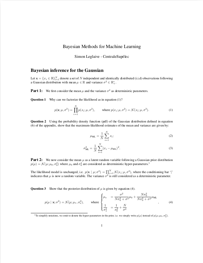![](images/exercise.png)]

---
class: middle, center
exclude: true

# Taking a step back and looking at the landscape of machine learning

---
exclude: true
class: middle

What we have seen so far actually corresponds to a subset of machine learning methods, involving
- **generative modeling**, because we define a generative model of the observed data; 
- **Bayesian modeling and inference**, because the generative model involves a latent random variable equiped with a prior and during inference we compute its posterior distribution;
- **unsupervised learning**, because the parameters of the model, which .italic[in fine] allow us to infer the latent variable of interest from the observations through the posterior, are learned from unlabeled data.

.alert-g[**Supervised learning** is another important subset of machine learning methods, which involves generative or **discriminative models**. This will be the topic of another lecture.]

---
exclude: true
class: middle

- Supervised learning with discriminative models is probably the dominating paradigm in machine learning, which has led to great research and industrial successes in recent years.

- But understanding first unsupervised learning with generative models greatly helps to have a deep understanding of supervised learning with discriminative models.

- This is for three reasons:

1. The whole story of extracting a latent variable of interest from observations is always valid **at test time**, whatever the machine learning method.
  2. Supervised learning is simply the case where, **at training time**, the variable of interest is not latent anymore but observed and used for the learning of the model parameters (no need to marginalize it anymore!);
  3. Discriminative modeling is simply the case where we directly define the posterior distribution in the modeling step, instead of defining the joint distribution and then using Bayes theorem.

---
exclude: true
class: middle

.center.width-90[![](images/unsupervised_supervised_ML.svg)]

.credit[Credits: [Antoine Deleforge](https://members.loria.fr/ADeleforge/lectures/), Inria, course given at Télécom Physique Strasbourg.]

---
exclude: true
class: middle
## Applications of unsupervised learning

.center.width-80[![](images/applications_unsupervised_learning.svg)]

.alert[Potential to learn from massive amount of unlabeled data to generate even more.]

.credit[Credits: [Antoine Deleforge](https://members.loria.fr/ADeleforge/lectures/), Inria, course given at Télécom Physique Strasbourg.]

---
exclude: true
class: middle
## Fundamental techniques in unsupervised learning

.center.width-80[![](images/fundamentals_unsupervised_learning.svg)]

These fundamental techniques can all be described from a probabilistic perspective, where 
- the structure of the latent variable of interest $z$ is encoded in a suitable probabilistic prior (**modeling**); 
- the task of extracting $z$ from the observations corresponds to the computation of its posterior (**inference**); 
- the model parameters are estimated by maximizing the marginal likelihood (**learning**).

We will study Bayesian/probabilistic methods for clustering and dim. reduction in this course.

.credit[Image credits: [Antoine Deleforge](https://members.loria.fr/ADeleforge/lectures/), Inria, course given at Télécom Physique Strasbourg.]

---
exclude: true
class: middle

The previous fundamental techniques form the basis of many advanced deep learning techniques used today:

- Variational autoencoders (VAEs);
- Generative adversarial networks (GANs);
- Normalizing flow;
- Diffusion models;
- Conditional neural processes;
- Self-supervised learning;
- etc.

.alert-g[This course is built as a journey towards a **deep understanding** of VAEs, which requires first to study **Bayesian modeling, inference, and learning methods**.]

---
class: center, middle

# The priors

---
class: middle

- The inference, and therefore the predictions, decisions and actions which are based on the inference (posterior computation) all depend on the prior.
- The prior summarizes the information you have about the latent variables of interest, as well as the uncertainty related to this information.
- The prior is a key ingredient to Bayesian inference, but it is not sufficient, you also need data.

.center[**How to convert prior information into prior distributions?**]

---
class: middle
## Conjugate priors

.alert-g[A familiy of probability distributions is conjugate for a likelihood function if for every prior in this family the posterior also belongs to this familiy. In other words, if the posterior distribution is in the same family as the prior distribution, **the prior is conjugate for the likelihood function**.]

- The "structure" of the prior is propagated to the posterior. Computing the posterior consists in **updating the prior parameters using the observations**.

- Using conjugate priors is **simple** and makes inference **tractable** (the marginal likelihood and therefore the posterior can be computed in closed form), but it is also **constraining**.

- For example, the Gaussian distribution is a conjugate prior for the Gaussian likelihood (with known variance); choosing a Gaussian prior over the mean will ensure that the posterior distribution is also Gaussian.

[Table of conjugate priors for various likelihood functions](https://en.wikipedia.org/wiki/Conjugate_prior#Table_of_conjugate_distributions).

---
class: middle
## Non-informative priors

- A non-informative or uninformative prior is a prior distribution which is designed to have a weak influence the posterior distribution.

- It is useful when we do not have any clear prior beliefs about the latent variables of interest, or we do not want these prior beliefs to influence the inference process.

- A non-informative prior typically yields results which are not too different from conventional statistical analysis, as the likelihood function often yields more information than the non-informative prior.

---
class: middle
## Uniform prior

The simplest and oldest rule (suggested by the pioneers of the Bayesian inference, Bayes and Laplace) for determining a non-informative prior is the principle of indifference, which assigns equal probabilities to all possibilities.

This rule leads a uniform prior:

- Discrete case: $p(z) = 1/K$ for $z \in \\{z\_1, ..., z\_K\\}$.
- Continuous case: $p(z) \propto 1$ (constant pdf).

The uniform prior does not influence the posterior:

$$ p(z | x) \propto p(x |z) p(z) \propto p(x |z). $$

---

- **The uniform prior is not invariant under reparametrization**:

If we have no information about $z$, we also have no information about $y = g(z) = 1/z$. But a uniform prior over $z$ does not correspond to a uniform prior over $1/z$. 
  
  By the change of variable formula:

$$ p\_Y(y) = p\_Z(g^{-1}(y)) \Big\lvert \frac{d}{dy} g^{-1}(y) \Big\rvert \propto y^{-2} \neq constant $$

- **The uniform prior is improper**:

If the random variable $z$ is real-valued, the uniform prior $p(z) \propto 1$ does not integrate to 1, we say that it is improper.

"Improperness" is not always a serious problem since improper priors can lead to proper posteriors.

- [Jeffreys' prior](https://en.wikipedia.org/wiki/Jeffreys_prior) is a proper and invariant under reparametrization non-informative prior.

---
exclude: true
## Jeffreys' prior

In the univariate (i.e. 1-dimensional) case, it is defined by:

$$ p(z) \propto \sqrt{I(z)}, $$

where $I(z)$ is the Fisher information:

$$ I(z) = \mathbb{E}\_{p(x | z)} \left[ \left(\frac{\partial \ln p(x | z)}{ \partial z} \right)^2 \right] = - \mathbb{E}\_{p(x | z)} \left[ \frac{\partial^2 \ln p(x | z)}{ \partial^2 z} \right], $$

with $p(x | z)$ is the likelihood.

In the multivariate case, the prior is proportional to the square root of the determinant of the Fisher information matrix.

---
exclude: true
Jeffreys' prior is invariant under reparametrization:

$$
\begin{aligned}
p\_Y(y) &= p\_Z(g^{-1}(y)) \Big\lvert \frac{d}{dy} g^{-1}(y) \Big\rvert\\\\
&\propto \sqrt{I(g^{-1}(y)) \left(\frac{d}{dy} g^{-1}(y)\right)^2}\\\\
&= \sqrt{\mathbb{E}\_{p(x | y)} \left[ \left(\frac{\partial \ln p(x | y)}{ \partial g^{-1}(y)} \right)^2 \right] \left(\frac{dg^{-1}(y)}{dy} \right)^2} \\\\
&= \sqrt{\mathbb{E}\_{p(x | y)} \left[ \left(\frac{\partial \ln p(x | y)}{ \partial g^{-1}(y)} \frac{dg^{-1}(y)}{dy} \right)^2 \right]} \\\\
&= \sqrt{\mathbb{E}\_{p(x | y)} \left[ \left(\frac{\partial \ln p(x | y)}{dy} \right)^2 \right]} \\\\
& = \sqrt{I(y)}.
\end{aligned}
$$

---
class: middle
## Hierarchical prior

- Considering a conjugate prior $p(z ; \theta\_z)$ may be too restrictive.

- Instead of treating $\theta\_z$ as a deterministic (hyper)parameters, we could consider it as another latent random variable, equipped with a prior $p(\theta\_z ; \lambda )$.

- The resulting prior over $z$ is hierarchical, i.e. it is expressed as a marginal distribution:

$$ p(z ; \gamma) = \int p(z, \theta\_z ; \gamma) d\theta\_z = \int p(z | \theta\_z) p(\theta\_z; \gamma) d\theta\,$$

- This prior is not conjugate anymore and it is "more expressive".

.vspace[

]

.footnote[What we treat as a (hyper)parameter or as a random variable is quite arbitrary and problem-dependent.]

---
class: middle

## Example: The Student's t distribution

$$\begin{cases}
p(z | v) &= \mathcal{N} \left(z; \mu, v \right) \\\\[.25cm]
p(v) &= \mathcal{IG}\left(v; \displaystyle \frac{\alpha}{2}, \frac{\alpha}{2} \lambda^2\right)
\end{cases}  \hspace{.5cm} \Leftrightarrow \hspace{.5cm}  p(z) = \int\_{0}^{+\infty} p(z | v) p(v) dv = \mathcal{T}_{\alpha}(z; \mu, \lambda)  $$
$$
- $\small \mathcal{N} \left(x; \mu, \sigma^2 \right) = \displaystyle \frac{1}{\sqrt{2\pi \sigma^2}} \exp\left[ \displaystyle \frac{(x-\mu)^2}{2\sigma^2} \right]$ .tiny[is the [Gaussian distribution](https://en.wikipedia.org/wiki/Normal_distribution) ].

- $\small \mathcal{IG}(x; \alpha, \beta) = \displaystyle \frac{\beta^\alpha}{\Gamma(\alpha)} x^{-(\alpha + 1)}\exp\left(-\beta/x\right) $ .tiny[ is the [inverse-gamma distribution](https://en.wikipedia.org/wiki/Inverse-gamma_distribution) ].

- $\small \mathcal{T}_{\alpha}(x; \mu, \lambda) = \displaystyle \frac{\Gamma(\frac{\alpha + 1}{2})}{\Gamma(\frac{\alpha}{2})\sqrt{\pi\alpha}\lambda\,} \left(1+\frac{1}{\alpha} \frac{ (x- \mu)^2 } {\lambda^2}\right)^{-\frac{\alpha+1}{2}}$ .tiny[is the [Student's t distribution](https://en.wikipedia.org/wiki/Student%27s_t-distribution#Generalized_Student's_t-distribution)].

.vspace[

]

.footnote[

.left-column[

Hints for the proof (exercise): 
- 1st change of variable: $ u = v \left( \frac{(x-u)^2}{2} + \frac{\alpha}{2}\lambda^2 \right) $

]

.right-column[
- 2nd change of variable: $ t = 1/u$
- Recognize the Gamma function $ \Gamma(z) = \int_0^\infty t^{z-1} e^{-t}\, dt$ for $z = (\alpha + 1)/2$.

]

---
exclude: true

.vspace[

.center[.width-80[![](images/studentsT_pdf_logy.svg)]]

]

It is a heavy-tailed distribution. It is more flexible than the Gaussian in the sense that it allows $x$ to take values that are "far from the mode".

---
## Natural image prior

.grid[

.kol-1-4[
  .center.width-100[![](images/cameraman.svg)]
  .caption[Image]
]
.kol-1-4[
  .center.width-100[![](images/cameraman_grad.svg)]
  .caption[Horizontal gradient]
]
.kol-1-2[
  .center.width-95[![](images/cameraman_gaussian_student_log.svg)]
  .caption[Empirical and estimated distribution of the gradient image]
]

]

- Bayesian image reconstruction methods (inpainting, denoising, deblurring) usually work on the gradient of the image and assume a Gaussian likelihood model. 
- The distribution of the gradient of natural images is sparse, which cannot be well represented by a simple Gaussian conjugate prior.
- Choosing a hierarchical Studen't t prior is much better, but it makes inference more difficult.

---
class: center, middle

.center.width-70[![](images/VB_image_deconv.png)]

---
class: center, middle
# Example applications of Bayesian methods

---
class: middle
## Kaggle contest on Observing Dark World

From [Observing Dark World](https://www.kaggle.com/c/DarkWorlds):

.block-center-70[
"There is more to the Universe than meets the eye. Out in the cosmos exists a form of matter that outnumbers the stuff we can see by almost 7 to 1, and we don’t know what it is. What we do know is that it does not emit or absorb light, so we call it Dark Matter. Such a vast amount of aggregated matter does not go unnoticed. In fact we observe that this stuff aggregates and forms massive structures called Dark Matter Halos. Although dark, it warps and bends spacetime such that any light from a background galaxy which passes close to the Dark Matter will have its path altered and changed. This bending causes the galaxy to appear as an ellipse in the sky."
]

The contest required predictions about where dark matter was likely to be. The winner, Tim Salimans, used Bayesian inference to find the best locations for the halos (interestingly, the second-place winner also used Bayesian inference).

---
class: middle

Tim Salimans' solution ([source](https://nbviewer.jupyter.org/github/CamDavidsonPilon/Probabilistic-Programming-and-Bayesian-Methods-for-Hackers/blob/master/Chapter5_LossFunctions/Ch5_LossFunctions_PyMC2.ipynb))
:

- Construct a prior distribution for the halo positions $p(z)$, i.e. formulate our expectations about the halo positions before looking at the data.
- Construct a probabilistic model for the data (observed ellipticities of the galaxies) given the positions of the dark matter halos: $p(x|z)$.
- Use Bayes’ rule to get the posterior distribution of the halo positions: $p(z|x)$, i.e. use the data to guess where the dark matter halos might be.
- Minimize the expected loss with respect to the posterior distribution over the predictions for the halo positions: $z^\star = \underset{\hat{z}}{\arg\min}\, \mathbb{E}\_{p(z|x)}[\mathcal{L}(\hat{z},z)]$ , i.e. tune our predictions to be as good as possible for the given error metric.

The loss function in this problem is very complicated, not something that can be written down in a single mathematical line.

---
class: middle

## Bayesian inference in gravitational-wave astronomy

.center.width-70[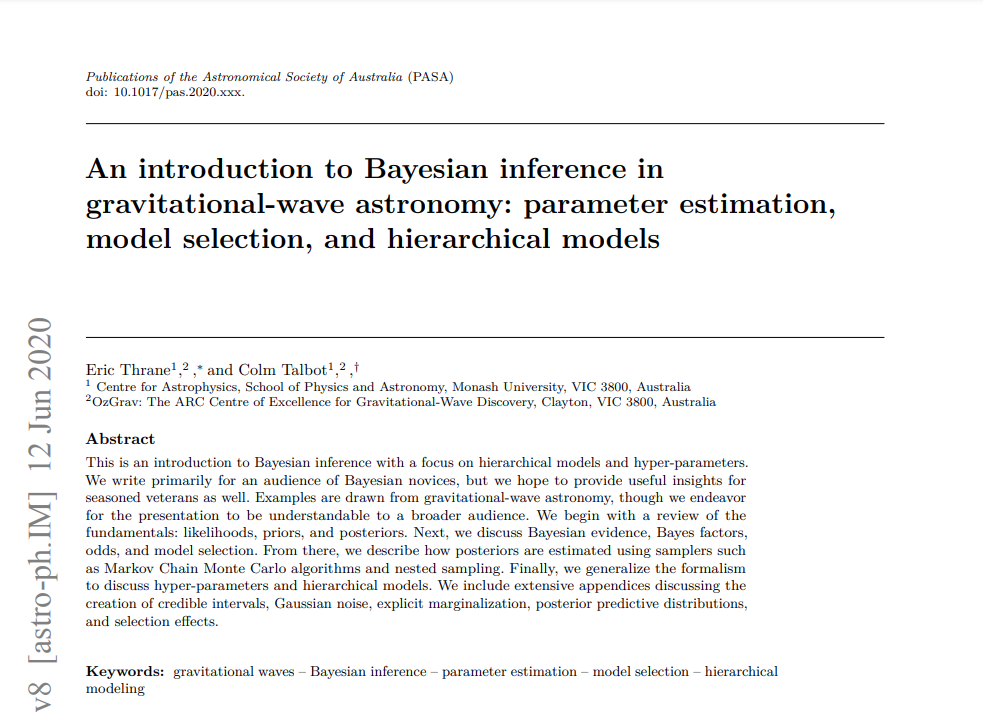![](images/grav_waves.png)]

---
class: middle

## Bayesian audio-visual multi-speaker tracking

.center[
<video width="700" controls>
 <source src="images/AVtracking.mp4" type="video/mp4">
</video>

]

.small[Y. Ban et al., Variational Bayesian Inference for Audio-Visual Tracking of Multiple Speakers, IEEE Transactions on Pattern Analysis and Machine Intelligence, 2019.]

---
class: middle

## Bayesian music source separation with a deep speech prior

.center[

.grid[

.kol-1-3[.center[Mix]]
.kol-1-3[.center[Vocals]]
.kol-1-3[.center[Accompaniment]]

.kol-1-3[<img src="audio/demo_music_sep/mix_spectro.svg", width=80%>]
.kol-1-3[<img src="audio/demo_music_sep/vocals_spectro.svg", width=80%>]
.kol-1-3[<img src="audio/demo_music_sep/accomp_spectro.svg", width=75%>]

]

.grid[

.kol-1-3[<img src="audio/demo_music_sep/mix_waveform.png", width=75%>]
.kol-1-3[<img src="audio/demo_music_sep/vocals_waveform.png", width=75%>]
.kol-1-3[<img src="audio/demo_music_sep/accomp_waveform.png", width=70%>]

]

.grid[

.kol-1-3[
<audio controls src="audio/demo_music_sep/mix.wav"></audio>
]
.kol-1-3[
<audio controls src="audio/demo_music_sep/vocals.wav"></audio>
]
.kol-1-3[
<audio controls src="audio/demo_music_sep/accomp.wav"></audio>
]

]

.small[S. Leglaive et al., 	A recurrent variational autoencoder for speech enhancement, IEEE ICASSP 2020.]

---
class: middle
## Bayesian topic modeling

.center.width-60[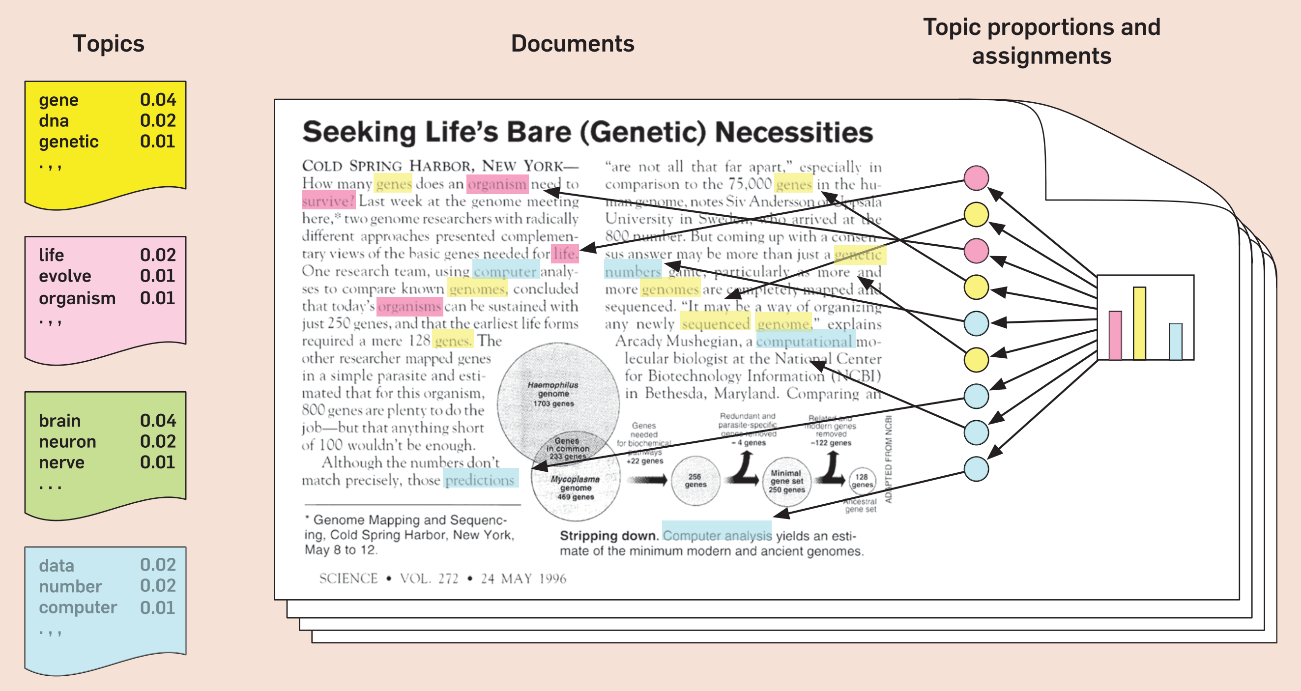![](images/LDA.png)]
.caption[Latent Dirichlet allocation. Credits: (Blei 2012).]

"[Latent Dirichlet allocation](https://en.wikipedia.org/wiki/Latent_Dirichlet_allocation) (LDA) is a generative probabilistic model of
a corpus. The basic idea is that documents are represented as random
mixtures over latent topics, where each topic is characterized by a
distribution over words." (Blei, Ng, and Jordan, 2003).

.credit[

Blei, D. M., Ng, A. Y., & Jordan, M. I. (2003). Latent dirichlet allocation. Journal of machine Learning research, 3(Jan), 993-1022.
 
Blei, D. (2012). Probabilistic Topic Models. Commun. ACM, 55(4), 77–84.

]
---
class: middle

## Conditional image generation with diffusion models

- Diffusion models are based on an efficient combination of deep learning and Bayesian techniques (Markov chain Monte Carlo, variational inference).

At the end of this course, you will have a sufficient backgroud in Bayesian methods to understand how diffusion models work, e.g. by reading [this paper](https://arxiv.org/pdf/2208.11970.pdf).

- Some recent models for text-to-image generation:
  - DALL•E 2 (6 Apr 2022)
  - Imagen (23 May 2022)
  - Stable Diffusion (22 Aug 2022)

- Why do we need a probabilistic approach for this task?

Because multiple images can correspond to one text prompt $\rightarrow$ we need to learn a conditional distribution over images, not a one-to-one mapping.

- Check out [this thread](https://twitter.com/daniel_eckler/status/1572210382944538624) on the rapid rise of stable diffusion.