class: center, middle <br/> # Bayesian Methods for Machine Learning .small-vspace[ ] ### Lecture 3 (part 2) - Inference in latent variable models <br/><br/> .bold[Simon Leglaive] <br/> <br/> <br/><br/> .tiny[CentraleSupélec] --- exclude: true .width-100.center[] .width-100.center[] --- ### Generative latent-variable model Let $\mathbf{x} \in \mathcal{X}$ and $\mathbf{z} \in \mathcal{Z}$ denote the **observed and latent** random variables, respectively. Developing a probabilistic model consists in defining the joint distribution of the observed and latent variables, also called **complete-data likelihood**: $$ p(\mathbf{x}, \mathbf{z}; \theta) = p(\mathbf{x} | \mathbf{z}; \theta) p(\mathbf{z}; \theta), $$ where $\theta$ is a set of **unknown deterministic parameters**. -- count: false Remarks: - $p(\mathbf{z}; \theta)$ is the **prior** over the latent variables. - $p(\mathbf{x} | \mathbf{z}; \theta)$ is the **likelihood**. - to simplify notations we use $\theta$ to denote both the parameters of the prior and likelihood, but these two distributions usually depend on disjoint sets of parameters. - In a full Bayesian setting, there are no deterministic parameters to be estimated. Parameters are also treated as latent variables and $\theta$ denotes **known and manually-fixed hyperparameters**. --- class: middle, center ## The two central problems in statistical inference for latent variable models --- class: middle ### Computing the posterior distribution of the latent variables .vspace[ ] $$ p(\mathbf{z} | \mathbf{x} ; \theta) = \frac{p(\mathbf{x} | \mathbf{z} ; \theta)p(\mathbf{z} ; \theta)}{p(\mathbf{x}; \theta)} = \frac{p(\mathbf{x} | \mathbf{z} ; \theta)p(\mathbf{z} ; \theta)}{\int p(\mathbf{x} | \mathbf{z} ; \theta)p(\mathbf{z} ; \theta) d\mathbf{z}}. $$ where $p(\mathbf{x}; {\theta}) = \int p(\mathbf{x} | \mathbf{z} ; \theta)p(\mathbf{z} ; \theta) d\mathbf{z}$ is the **marginal likelihood**, also called evidence. .vspace[ ] - Computing this posterior is the **inference** step. - The posterior summarizes our knowledge on latent variables of interest, once we have observed the data. - For numerous probabilistic models, the posterior is analytically intractable, e.g. because its normalizing constant – the marginal likelihood – cannot be computed analytically. --- class: middle ### Estimating the model parameters by maximum (marginal) likelihood .vspace[ ] $$ \hat{\theta} = \underset{\theta}{\arg\max}\hspace{.2cm} p(\mathbf{x}; {\theta}) = \underset{{\theta}}{\arg\max} \int p(\mathbf{x} | \mathbf{z} ; {\theta})p(\mathbf{z} ; {\theta}) d\mathbf{z}.$$ .vspace[ ] - Solving this optimization problem is the **learning** step. - Quite often, directly solving the optimization problem associated with this ML estimation procedure is difficult, if not impossible when the marginal likelihood cannot be computed analytically. --- class: middle Today, we will focus on models where directly maximizing the likelihood is difficult, but the posterior distribution of the latent variables can be computed analytically. --- class: middle These two problems (parameters estimation and posterior inference) are actually strongly related: 1. the posterior distribution of the latent variables depends on the model parameters. 2. as we are going to see, when direct maximization of the marginal likelihood is impossible, we usually consider the maximization of a lower bound, which precisely depends on the posterior distribution of the latent variables. --- class: center, middle ## Illustrative example .block-center-70[ .medium.center[The following example and drawings are adapted from a [tutorial on Bayesian Learning for Signal Processing](https://members.loria.fr/ADeleforge/files/bayesian_inference_electronic.pdf) given by Antoine Deleforge at the LVA/ICA 2015 Summer School.] ] --- class: center, middle  .left.credit[Image credit: Antoine Deleforge, [Tutorial on Bayesian Learning for Signal Processing](https://members.loria.fr/ADeleforge/files/bayesian_inference_electronic.pdf), LVA/ICA 2015 Summer School] --- class: center, middle  .left.credit[Image credit: Antoine Deleforge, [Tutorial on Bayesian Learning for Signal Processing](https://members.loria.fr/ADeleforge/files/bayesian_inference_electronic.pdf), LVA/ICA 2015 Summer School] --- class: center, middle  .left.credit[Image credit: Antoine Deleforge, [Tutorial on Bayesian Learning for Signal Processing](https://members.loria.fr/ADeleforge/files/bayesian_inference_electronic.pdf), LVA/ICA 2015 Summer School] --- class: center, middle  .left.credit[Image credit: Antoine Deleforge, [Tutorial on Bayesian Learning for Signal Processing](https://members.loria.fr/ADeleforge/files/bayesian_inference_electronic.pdf), LVA/ICA 2015 Summer School] --- class: middle, center ### Modeling --- .left-column[ **Observed variables**: $ \\{\mathbf{x}\_n \in \mathbb{R}^2\\}\_{n=1}^N$. .width-80.center[] ** Bayesian network** .width-50.center[] $$ p(\\{\mathbf{x}\_n, z\_n\\}\_{n=1}^N; \theta) = \prod\nolimits\_{n=1}^N p(\mathbf{x}\_n | z\_n; \theta) p(z\_n; \theta). $$ ] .right-column[ **Hidden variables**: $ \\{z\_n \in \\{1,2,3\\} \\}\_{n=1}^N$. .width-90.center[] ] --- .grid[ .kol-1-2[ .vspace[ ] .width-50.center[] ] .kol-1-2[ .width-70.center[] ] .kol-1-4[ **Prior** ] .kol-3-4[ $ p(z\_n = k; \theta) = \pi\_k, \qquad \sum\_{k=1}^K \pi\_k = 1, \qquad K=3$ ] .kol-1-4[ **Likelihood** ] .kol-3-4[ $ p(\mathbf{x}\_n | z\_n=k ; \theta) = \mathcal{N}\left(\mathbf{x}\_n; \boldsymbol{\mu}\_k, \boldsymbol{\Sigma}\_k \right)$ ] .kol-1-4[ **Parameters** ] .kol-3-4[ $\theta = \\{\pi\_k, \boldsymbol{\mu}\_k, \boldsymbol{\Sigma}\_k \\}\_{k=1}^K.$ ] ] --- **Marginal likelihood** $$ \begin{aligned} p(\\{\mathbf{x}\_n\\}\_{n=1}^N; \theta) &= \prod\_{n=1}^N p(\mathbf{x}\_n ; \theta) \\\\ &= \prod\_{n=1}^N \sum\_{k=1}^{K} p(\mathbf{x}\_n | z\_n = k ; \theta) p(z\_n = k; \theta) \\\\ &= \prod\_{n=1}^N \sum\_{k=1}^{K} \pi\_k \mathcal{N}\left(\mathbf{x}\_n; \boldsymbol{\mu}\_k, \boldsymbol{\Sigma}\_k \right). \end{aligned} $$ Observations are independent and identically distributed according to a **Gaussian mixture model** (GMM) with $K=3$ components. The parameters $\pi\_k$ are called the **mixing coefficients**, they give the prior probability of picking the k-th component to generate a data point $\mathbf{x}\_n$. ??? $$ \begin{aligned} p(\mathbf{x}\_1, \mathbf{x}\_2) &= \sum\_{j, k} p(\mathbf{x}\_1, \mathbf{x}\_2, z\_1=j, z\_2=k) \\\\ &= \sum\_{j, k} p(\mathbf{x}\_1| z\_1=j) p(z\_1=j) p(\mathbf{x}\_2 | z\_2=k) p(z\_2=k) \\\\ &= \sum\_{j} \left[ \sum\_{k} p(\mathbf{x}\_1| z\_1=j) p(z\_1=j) p(\mathbf{x}\_2 | z\_2=k) p(z\_2=k) \right] \\\\ &= \sum\_{j} p(\mathbf{x}\_1| z\_1=j) p(z\_1=j) \left[ \sum\_{k} p(\mathbf{x}\_2 | z\_2=k) p(z\_2=k) \right] \\\\ &= p(\mathbf{x}\_1) p(\mathbf{x}\_2) \\\\ \end{aligned} $$ --- class: middle, center ### Inference --- **Posterior distribution** .grid[ .kol-1-2[ $ p(\\{z\_n\\}\_{n=1}^N | \\{\mathbf{x}\_n\\}\_{n=1}^N; \theta) = \prod\_{n=1}^N p(z\_n | \mathbf{x}\_n; \theta), $ where $ \begin{aligned} p(z\_n = k | \mathbf{x}\_n; \theta) &= \frac{ p(\mathbf{x}\_n | z\_n = k; \theta) p(z\_n = k; \theta) }{p(\mathbf{x}\_n ; \theta)} \\\\[.3cm] &= \frac{ p(\mathbf{x}\_n | z\_n = k; \theta) p(z\_n = k; \theta) }{\sum\_{j=1}^K p(\mathbf{x}\_n | z\_n = j; \theta) p(z\_n = j; \theta) } \\\\[.5cm] &= \frac{ \pi\_k p(\mathbf{x}\_n | z\_n = k; \theta) }{\sum\_{j=1}^K \pi\_j p(\mathbf{x}\_n | z\_n = j; \theta) }. \end{aligned} $ ] .kol-1-2[ .width-90.right[] ] ] The posterior probabilities $p(z\_n = k | \mathbf{x}\_n; \theta)$ are also known as the **responsabilities**. The argmax of the responsability assigns the observation to a component, i.e. it **clusters the data**. --- **Parameters estimation** The posterior distribution can be computed analytically, but it depends on the **unknown model parameters** $\theta = \\{\pi\_k, \boldsymbol{\mu}\_k, \boldsymbol{\Sigma}\_k \\}\_{k=1}^K$. Ideally, we would like to estimate them by maximizing the log-marginal likelihood: $$ \begin{aligned} \mathcal{L}(\theta) &= \ln p(\\{\mathbf{x}\_n\\}\_{n=1}^N; \theta) \\\\ &= \ln \prod\_{n=1}^N \sum\_{k=1}^{K} \pi\_k \mathcal{N}\left(\mathbf{x}\_n; \boldsymbol{\mu}\_k, \boldsymbol{\Sigma}\_k \right) \\\\ &= \sum\_{n=1}^N \ln \left(\sum\_{k=1}^{K} \pi\_k \mathcal{N}\left(\mathbf{x}\_n; \boldsymbol{\mu}\_k, \boldsymbol{\Sigma}\_k \right) \right). \end{aligned}$$ Due to the presence of the sum over $k$ inside the logarithm, **the maximum marginal likelihood solution for the parameters does not have a closed-form analytical solution.** --- count: false class: center, middle .width-90.center[] --- class: center, middle ## The expectation-maximization algorithm --- class: middle The expectation-maximization (EM) algorithm is a general technique introduced by Dempster et al. in 1977 for maximum likelihood parameters estimation in probabilistic models having latent variables. Let $\mathbf{x} \in \mathcal{X}$ and $\mathbf{z} \in \mathcal{Z}$ denote the **observed and latent** random variables, respectively, which are assumed to be continuous, although the discussion is identical in the discrete setting. We assume that direct optimization of the marginal likelihood $p(\mathbf{x}; {\theta})$ is difficult, while optimization of the complete-data likelihood function $p(\mathbf{x}, \mathbf{z} ; \theta)$ is much simpler. --- ### The evidence lower bound We first introduce a distribution over the latent variables whose probability density function is denoted by $q(\mathbf{z})$. For any distribution $q(\mathbf{z})$, the following decomposition of the log-marginal likelihood holds: $$ \ln p(\mathbf{x}; \theta) = \mathcal{L}(q(\mathbf{z}), \theta) + D\_{\text{KL}}(q(\mathbf{z} ) \parallel p(\mathbf{z} | \mathbf{x}; \theta)),$$ where $\mathcal{L}(q(\mathbf{z}), \theta)$ is called the **evidence lower bound** (ELBO), and it is defined by $$ \mathcal{L}(q(\mathbf{z}), \theta) = \mathbb{E}\_{q(\mathbf{z})} [\ln p(\mathbf{x}, \mathbf{z}; \theta) - \ln q(\mathbf{z} )]. $$ The **Kullback-Leibler** (KL) divergence is defined by: $$D\_{\text{KL}}(q \parallel p) = \mathbb{E}\_{q}[ \ln(q) - \ln(p)],$$ and it satisfies $D\_{\text{KL}}(q \parallel p) \ge 0$ with equality if and only if $q = p$. --- .tiny[Proof:] $\scriptsize \ln p(\mathbf{x}; \theta) = \mathbb{E}\_{q(\mathbf{z})}[\ln p(\mathbf{x}; \theta)] = \mathbb{E}\_{q(\mathbf{z})}[\ln p(\mathbf{x}, \mathbf{z}; \theta) - \ln p(\mathbf{z} | \mathbf{x}; \theta) - \ln q(\mathbf{z}) + \ln q(\mathbf{z}) ] $ --- $$ \ln p(\mathbf{x}; \theta) = \mathcal{L}(q(\mathbf{z}), \theta) + D\_{\text{KL}}(q(\mathbf{z} ) \parallel p(\mathbf{z} | \mathbf{x}; \theta))$$ <hr> As the KL divergence is always non-negative, we have: $$\ln p(\mathbf{x}; \theta) \ge \mathcal{L}(q(\mathbf{z}), \theta), $$ with equality if and only if $q(\mathbf{z}) = p(\mathbf{z} | \mathbf{x}; \theta)$. The ELBO is indeed a **lower bound of the log-marginal likelihood**, which is tight if $q(\mathbf{z})$ matches the true posterior. .width-40.center[] .credit[Image credit: Christopher M. Bishop, [Pattern Recognition and Machine Learning](https://www.microsoft.com/en-us/research/uploads/prod/2006/01/Bishop-Pattern-Recognition-and-Machine-Learning-2006.pdf), Springer, 2006.] --- ### EM algorithm The EM algorithm is an iterative algorithm which alternates between optimizing the ELBO with respect to $q$ in the E-Step and with repspect to $\theta$ in the M-step. We first **initialize** $\theta\_0$, then we iterate for $t \ge 0$ - **E-Step**: $ q\_{t+1}(\mathbf{z}) = \underset{q}{\arg\max}\, \mathcal{L}(q(\mathbf{z}), \theta\_{t}) $ - **M-Step**: $ \theta\_{t+1} = \underset{\theta}{\arg\max}\, \mathcal{L}(q\_{t+1}(\mathbf{z}), \theta) $ --- ### E-Step We recall the decomposition of the log-marginal likelihood: $$ \ln p(\mathbf{x}; \theta) = \mathcal{L}(q(\mathbf{z}), \theta) + D\_{\text{KL}}(q(\mathbf{z} ) \parallel p(\mathbf{z} | \mathbf{x}; \theta)).$$ The solution of the E-step is given by: $$ \begin{aligned} q\_{t+1}(\mathbf{z}) &= \underset{q}{\arg\max}\, \mathcal{L}(q(\mathbf{z}), \theta\_{t}) \\\\[.5cm] &= \underset{q}{\arg\min}\, D\_{\text{KL}}(q(\mathbf{z} ) \parallel p(\mathbf{z} | \mathbf{x}; \theta\_{t})) \\\\[.5cm] &= p(\mathbf{z} | \mathbf{x}; \theta\_{t}). \end{aligned} $$ --- class: middle After the E-Step, we have $D\_{\text{KL}}(q\_{t+1}(\mathbf{z} ) \parallel p(\mathbf{z} | \mathbf{x}; \theta\_{t})) = 0$, and the ELBO is equal to the log-marginal likelihood (i.e. the lower-bound is tight): $$ \ln p(\mathbf{x}; \theta\_t) = \mathcal{L}(q\_{t+1}(\mathbf{z}), \theta\_t). $$ .small-vspace[ ] .width-50.center[] Therefore, maximizing the lower-bound with respect to the model parameters in the M-step will necessarily increase the log-marginal likelihood. .credit[Image credit: Christopher M. Bishop, [Pattern Recognition and Machine Learning](https://www.microsoft.com/en-us/research/uploads/prod/2006/01/Bishop-Pattern-Recognition-and-Machine-Learning-2006.pdf), Springer, 2006.] --- ### M-Step - We recall the expression of the ELBO: $$ \mathcal{L}(q(\mathbf{z}), \theta) = \mathbb{E}\_{q(\mathbf{z})} [\ln p(\mathbf{x}, \mathbf{z}; \theta) - \ln q(\mathbf{z} )], $$ - The solution of the M-step is given by: $$ \begin{aligned} \theta\_{t+1} &= \underset{\theta}{\arg\max}\, \mathcal{L}(q\_{t+1}(\mathbf{z}), \theta) \\\\[.5cm] &= \underset{\theta}{\arg\max}\, \mathcal{L}\big( p(\mathbf{z} | \mathbf{x}; \theta\_{t}), \theta\big) \\\\[.5cm] &= \underset{\theta}{\arg\max}\, \mathbb{E}\_{ p(\mathbf{z} | \mathbf{x}; \theta\_{t})} [\ln p(\mathbf{x}, \mathbf{z}; \theta) - \ln p(\mathbf{z} | \mathbf{x}; \theta\_{t})] \\\\[.5cm] &= \underset{\theta}{\arg\max}\, \mathbb{E}\_{ p(\mathbf{z} | \mathbf{x}; \theta\_{t})} [\ln p(\mathbf{x}, \mathbf{z}; \theta) ] + cst(\theta), \end{aligned} $$ where the constant is the differential entropy of $p(\mathbf{z} | \mathbf{x}; \theta\_{t})$ which is independent of $\theta$. --- .footnote[We recall the decomposition of the log-marginal likelihood $ \ln p(\mathbf{x}; \theta) = \mathcal{L}(q(\mathbf{z}), \theta) + D\_{\text{KL}}(q(\mathbf{z} ) \parallel p(\mathbf{z} | \mathbf{x}; \theta)).$] After the M-step, because $q\_{t+1}(\mathbf{z} ) = p(\mathbf{z} | \mathbf{x}; \theta\_{t})$ has been held fixed for computing the new model parameters $\theta\_{t+1}$, the KL divergence $D\_{\text{KL}}(q\_{t+1}(\mathbf{z} ) \parallel p(\mathbf{z} | \mathbf{x}; \theta\_{t+1}))$ will be non zero. The increase in the log-marginal likelihood function is therefore greater than the increase in the ELBO, as shown below. .width-40.center[] .credit[Image credit: Christopher M. Bishop, [Pattern Recognition and Machine Learning](https://www.microsoft.com/en-us/research/uploads/prod/2006/01/Bishop-Pattern-Recognition-and-Machine-Learning-2006.pdf), Springer, 2006.] --- .grid[ .kol-1-3[ Initialize $\theta\_0$. ] .kol-2-3[ .width-90.right[] ] ] --- count: false .grid[ .kol-1-3[ Iteration $t=1$: - **E-Step**: $\qquad q\_{1}(\mathbf{z}) = p(\mathbf{z} | \mathbf{x}; \theta\_0)$ ] .kol-2-3[ .width-90.right[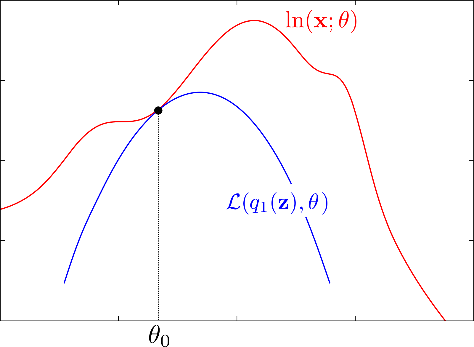] ] ] We have $D\_{\text{KL}}(q\_{1}(\mathbf{z}) \parallel p(\mathbf{z} | \mathbf{x}; \theta\_{0})) = 0 $ such that $\ln p(\mathbf{x}; \theta\_0) = \mathcal{L}(q\_{1}(\mathbf{z}), \theta\_0)$. --- count: false .grid[ .kol-1-3[ Iteration $t=1$: - E-Step: $\qquad q\_{1}(\mathbf{z}) = p(\mathbf{z} | \mathbf{x}; \theta\_0)$ - **M-Step**: $\theta\_1 = \underset{\theta}{\arg\max}\, \mathcal{L}(q\_{1}(\mathbf{z}), \theta) $ ] .kol-2-3[ .width-90.right[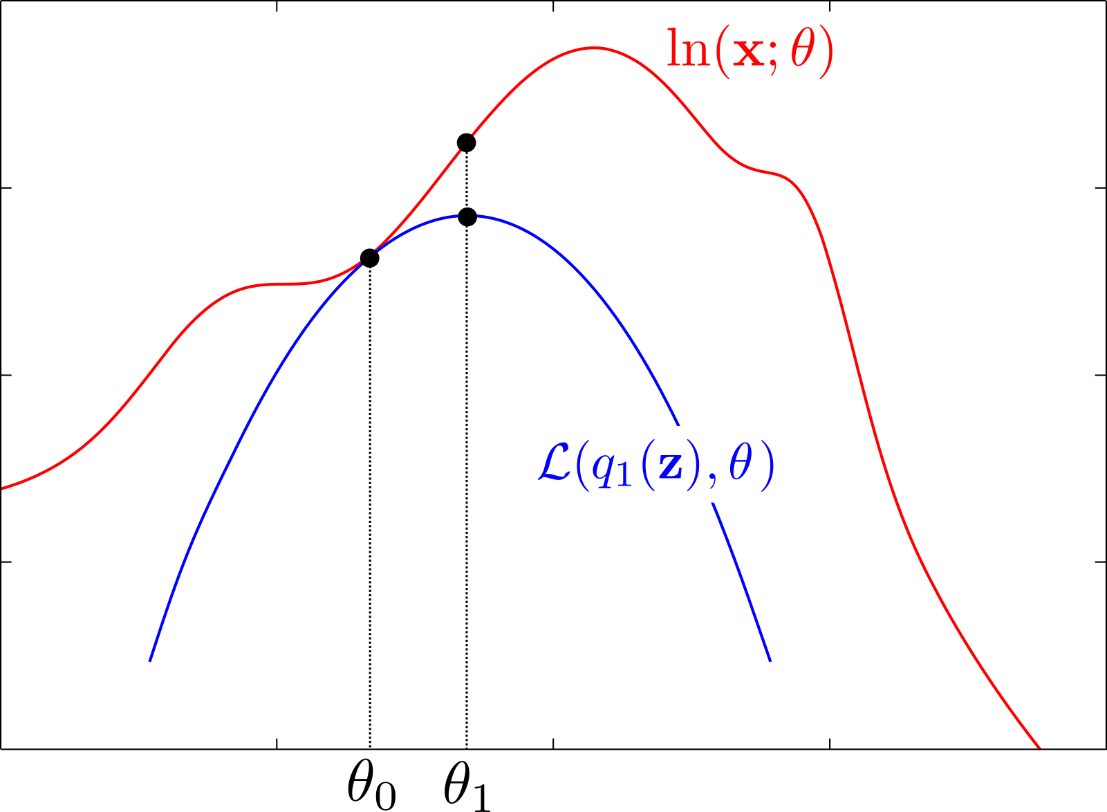] ] ] --- count: false .grid[ .kol-1-3[ Iteration $t=1$: - E-Step: $\qquad q\_{1}(\mathbf{z}) = p(\mathbf{z} | \mathbf{x}; \theta\_0)$ - M-Step: $\theta\_1 = \underset{\theta}{\arg\max}\, \mathcal{L}(q\_{1}(\mathbf{z}), \theta) $ ] .kol-2-3[ .width-90.right[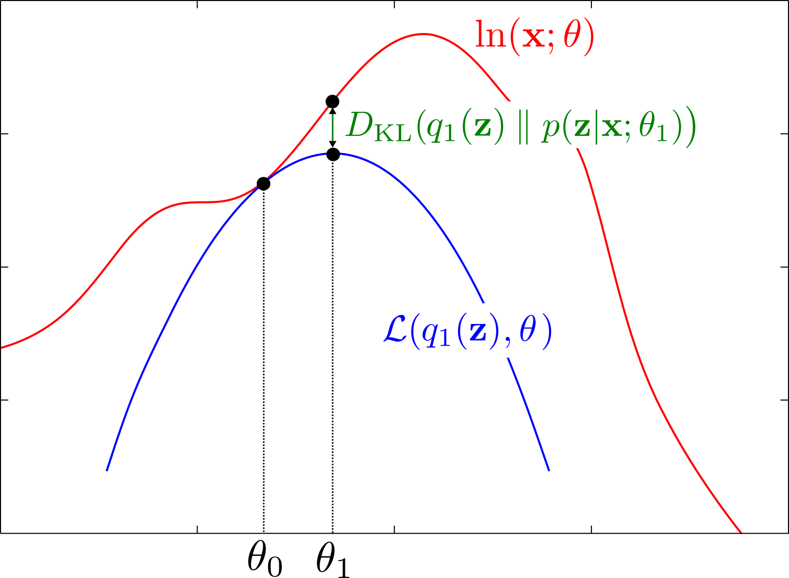] ] ] We have $D\_{\text{KL}}(q\_{1}(\mathbf{z} ) \parallel p(\mathbf{z} | \mathbf{x}; \theta\_{1})) \neq 0$. --- count: false .grid[ .kol-1-3[ Iteration $t=2$: - **E-Step**: $\qquad q\_{2}(\mathbf{z}) = p(\mathbf{z} | \mathbf{x}; \theta\_1)$ ] .kol-2-3[ .width-90.right[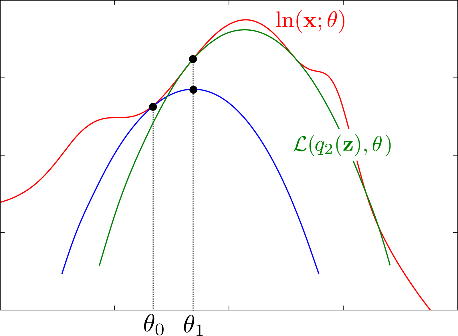] ] ] We have $D\_{\text{KL}}(q\_{2}(\mathbf{z}) \parallel p(\mathbf{z} | \mathbf{x}; \theta\_{1})) = 0 $ such that $\ln p(\mathbf{x}; \theta\_1) = \mathcal{L}(q\_{2}(\mathbf{z}), \theta\_1)$. --- count: false .grid[ .kol-1-3[ Iteration $t=2$: - E-Step: $\qquad q\_{2}(\mathbf{z}) = p(\mathbf{z} | \mathbf{x}; \theta\_1)$ - **M-Step**: $\theta\_2 = \underset{\theta}{\arg\max}\, \mathcal{L}(q\_{2}(\mathbf{z}), \theta) $ ] .kol-2-3[ .width-90.right[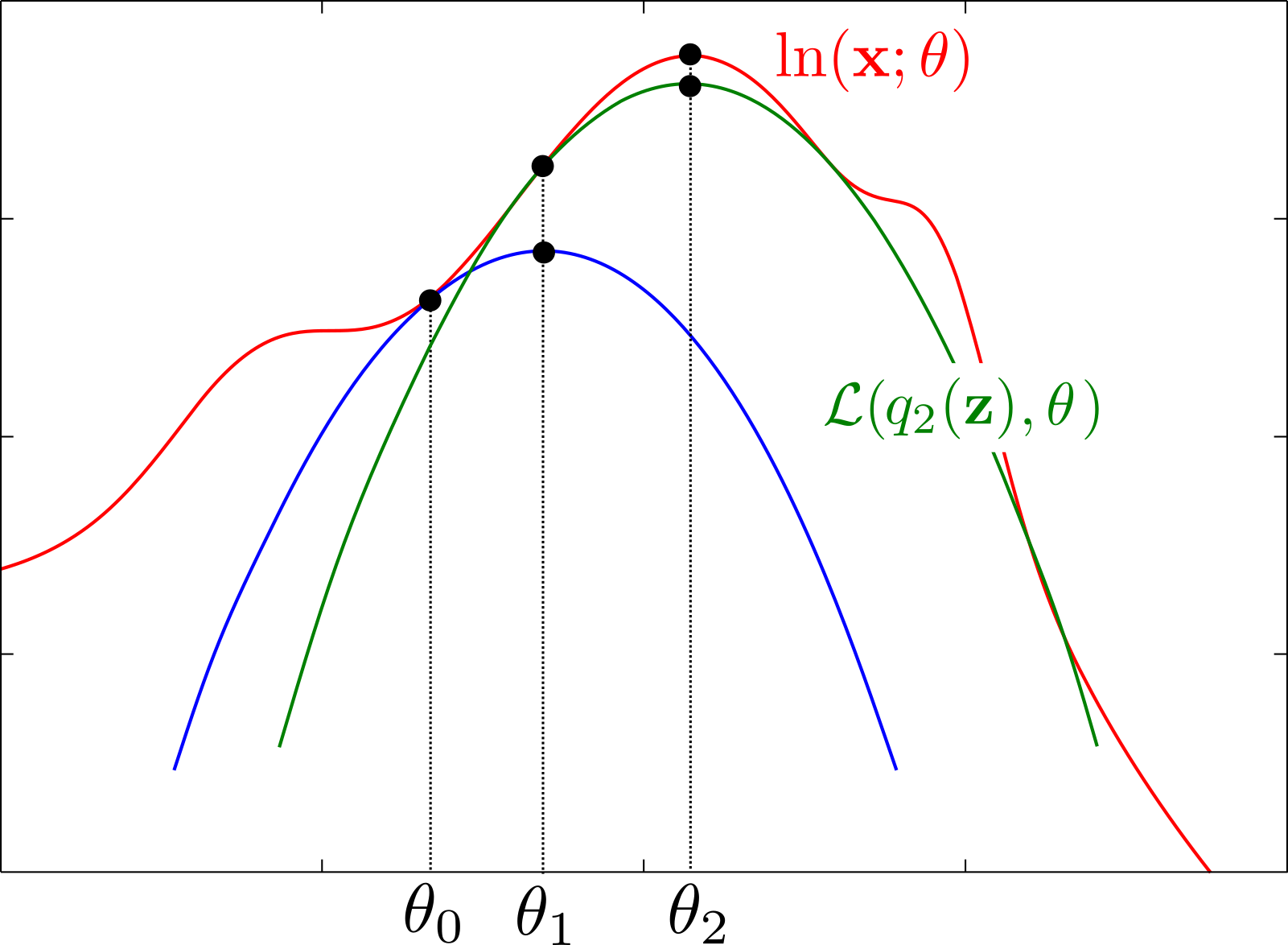] ] ] --- count: false .grid[ .kol-1-3[ Iteration $t=2$: - E-Step: $\qquad q\_{2}(\mathbf{z}) = p(\mathbf{z} | \mathbf{x}; \theta\_1)$ - M-Step: $\theta\_2 = \underset{\theta}{\arg\max}\, \mathcal{L}(q\_{2}(\mathbf{z}), \theta) $ - **We reached a stationary point.** ] .kol-2-3[ .width-90.right[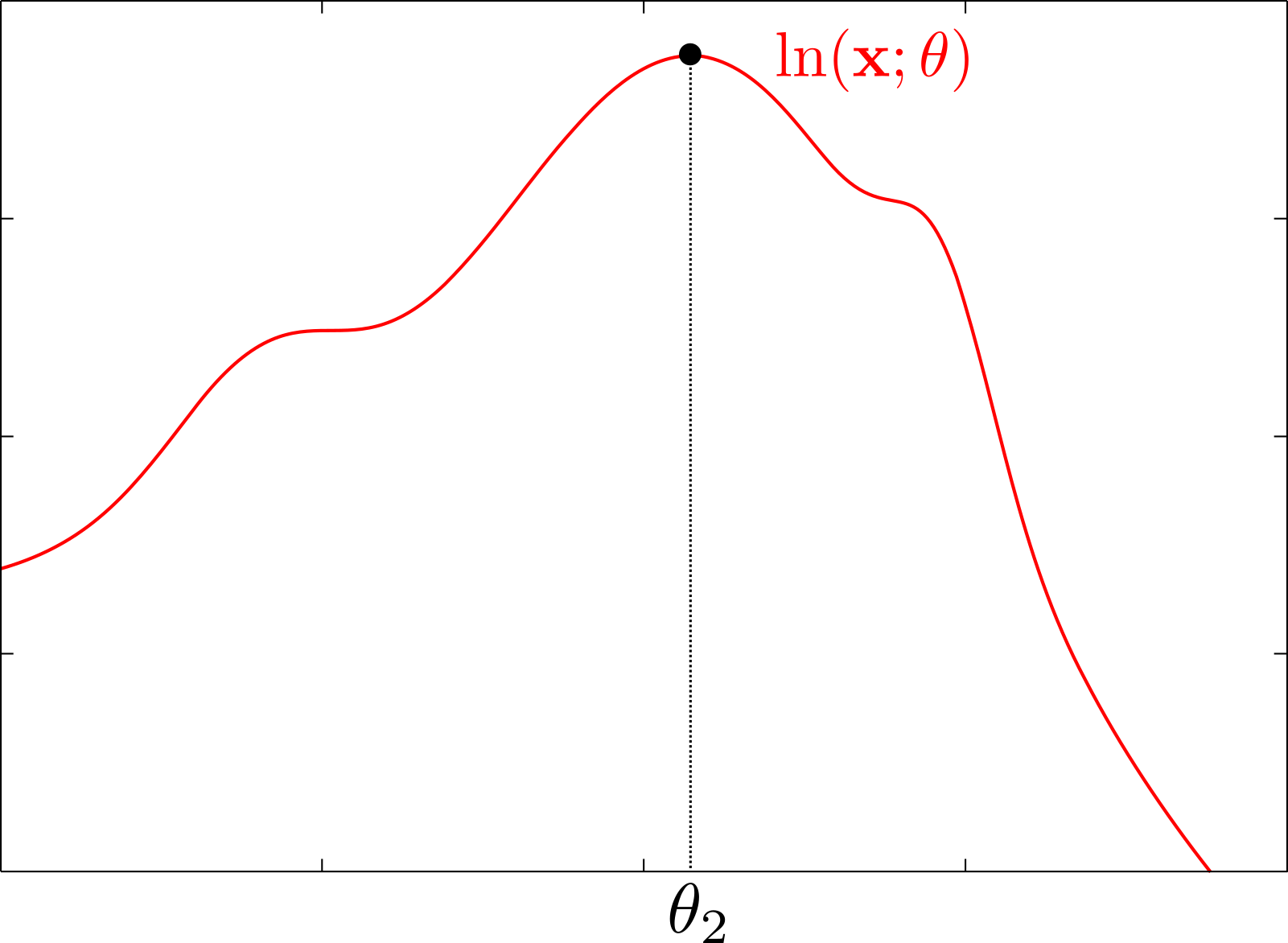] ] ] --- ### Properties of the EM algorithm - The log-marginal likelihood is **monotonically increasing**. -- count: false --- .bold[Proof]: Using the fact that $ \ln p(\mathbf{x}; \theta) = \mathcal{L}(q(\mathbf{z}), \theta) + D\_{\text{KL}}(q(\mathbf{z} ) \parallel p(\mathbf{z} | \mathbf{x}; \theta))$ and $q\_{t+1}(\mathbf{z}) = p(\mathbf{z} | \mathbf{x}; \theta\_{t})$ we deduce: $$\mathcal{L}(q\_{t+1}(\mathbf{z}), \theta\_{t}) = \ln p(\mathbf{x}; \theta\_{t}),$$ $$\mathcal{L}(q\_{t+1}(\mathbf{z}), \theta\_{t+1}) \le \ln p(\mathbf{x}; \theta\_{t+1}). $$ Moreover, by definintion of the M-step: $$\mathcal{L}(q\_{t+1}(\mathbf{z}), \theta\_{t+1}) \ge \mathcal{L}(q\_{t+1}(\mathbf{z}), \theta\_{t}). $$ Putting all together we have: $$ \ln p(\mathbf{x}; \theta\_{t+1}) \ge \mathcal{L}(q\_{t+1}(\mathbf{z}), \theta\_{t+1}) \ge \mathcal{L}(q\_{t+1}(\mathbf{z}), \theta\_{t}) = \ln p(\mathbf{x}; \theta\_{t}). $$ --- --- count: false ### Properties of the EM algorithm - The log-marginal likelihood is **monotonically increasing**. - The algorithm converges to a **stationary point** of the log-marginal likelihood. - As the problem is generally not convex, the algorithm generally converges to a local optimum which strongly **depends on the initialization**. --- ### EM algorithm summary The EM algorithm can be reformulated in the space of the model parameters only. Given an initialization $\theta\_0$ of the model parameters, iterate for $t=0:T-1$: - **E-Step**: $Q(\theta, \theta\_t) = \mathbb{E}\_{ p(\mathbf{z} | \mathbf{x}; \theta\_{t})} [\ln p(\mathbf{x}, \mathbf{z}; \theta) ]$; - **M-Step**: $\theta\_{t+1} = \underset{\theta}{\arg\max}\, Q(\theta, \theta\_t) $. .bold[This is the recipe you should remember and use to derive an EM algorithm.] --- ## Back to the adventures of Thomas Bayes .width-90.center[] --- class: middle .grid[ .kol-1-2[  ] .kol-1-2[ - Initialization: Random "guess" for $\theta\_0$ - E-Step: $Q(\theta, \theta\_t) = \mathbb{E}\_{ p(\mathbf{z} | \mathbf{x}; \theta\_{t})} [\ln p(\mathbf{x}, \mathbf{z}; \theta) ]$ - M-Step: $\theta\_{t+1} = \arg\max\_\theta\, Q(\theta, \theta\_t) $ - Convergence ] ] .left.credit[Image credit: Antoine Deleforge, [Tutorial on Bayesian Learning for Signal Processing](https://members.loria.fr/ADeleforge/files/bayesian_inference_electronic.pdf), LVA/ICA 2015 Summer School] --- class: middle count: false .grid[ .kol-1-2[  ] .kol-1-2[ - **Initialization**: Random "guess" for $\theta\_0$ - E-Step: $Q(\theta, \theta\_t) = \mathbb{E}\_{ p(\mathbf{z} | \mathbf{x}; \theta\_{t})} [\ln p(\mathbf{x}, \mathbf{z}; \theta) ]$ - M-Step: $\theta\_{t+1} = \arg\max\_\theta\, Q(\theta, \theta\_t) $ - Convergence ] ] .left.credit[Image credit: Antoine Deleforge, [Tutorial on Bayesian Learning for Signal Processing](https://members.loria.fr/ADeleforge/files/bayesian_inference_electronic.pdf), LVA/ICA 2015 Summer School] --- class: middle count: false .grid[ .kol-1-2[  ] .kol-1-2[ - Initialization: Random "guess" for $\theta\_0$ - **E-Step**: $Q(\theta, \theta\_t) = \mathbb{E}\_{ p(\mathbf{z} | \mathbf{x}; \theta\_{t})} [\ln p(\mathbf{x}, \mathbf{z}; \theta) ]$ - M-Step: $\theta\_{t+1} = \arg\max\_\theta\, Q(\theta, \theta\_t) $ - Convergence ] ] .left.credit[Image credit: Antoine Deleforge, [Tutorial on Bayesian Learning for Signal Processing](https://members.loria.fr/ADeleforge/files/bayesian_inference_electronic.pdf), LVA/ICA 2015 Summer School] --- class: middle count: false .grid[ .kol-1-2[  ] .kol-1-2[ - Initialization: Random "guess" for $\theta\_0$ - E-Step: $Q(\theta, \theta\_t) = \mathbb{E}\_{ p(\mathbf{z} | \mathbf{x}; \theta\_{t})} [\ln p(\mathbf{x}, \mathbf{z}; \theta) ]$ - **M-Step**: $\theta\_{t+1} = \arg\max\_\theta\, Q(\theta, \theta\_t) $ - Convergence ] ] .left.credit[Image credit: Antoine Deleforge, [Tutorial on Bayesian Learning for Signal Processing](https://members.loria.fr/ADeleforge/files/bayesian_inference_electronic.pdf), LVA/ICA 2015 Summer School] --- class: middle count: false .grid[ .kol-1-2[  ] .kol-1-2[ - Initialization: Random "guess" for $\theta\_0$ - **E-Step**: $Q(\theta, \theta\_t) = \mathbb{E}\_{ p(\mathbf{z} | \mathbf{x}; \theta\_{t})} [\ln p(\mathbf{x}, \mathbf{z}; \theta) ]$ - M-Step: $\theta\_{t+1} = \arg\max\_\theta\, Q(\theta, \theta\_t) $ - Convergence ] ] .left.credit[Image credit: Antoine Deleforge, [Tutorial on Bayesian Learning for Signal Processing](https://members.loria.fr/ADeleforge/files/bayesian_inference_electronic.pdf), LVA/ICA 2015 Summer School] --- class: middle count: false .grid[ .kol-1-2[  ] .kol-1-2[ - Initialization: Random "guess" for $\theta\_0$ - E-Step: $Q(\theta, \theta\_t) = \mathbb{E}\_{ p(\mathbf{z} | \mathbf{x}; \theta\_{t})} [\ln p(\mathbf{x}, \mathbf{z}; \theta) ]$ - **M-Step**: $\theta\_{t+1} = \arg\max\_\theta\, Q(\theta, \theta\_t) $ - Convergence ] ] .left.credit[Image credit: Antoine Deleforge, [Tutorial on Bayesian Learning for Signal Processing](https://members.loria.fr/ADeleforge/files/bayesian_inference_electronic.pdf), LVA/ICA 2015 Summer School] --- class: middle count: false .grid[ .kol-1-2[  ] .kol-1-2[ - Initialization: Random "guess" for $\theta\_0$ - **E-Step**: $Q(\theta, \theta\_t) = \mathbb{E}\_{ p(\mathbf{z} | \mathbf{x}; \theta\_{t})} [\ln p(\mathbf{x}, \mathbf{z}; \theta) ]$ - M-Step: $\theta\_{t+1} = \arg\max\_\theta\, Q(\theta, \theta\_t) $ - Convergence ] ] .left.credit[Image credit: Antoine Deleforge, [Tutorial on Bayesian Learning for Signal Processing](https://members.loria.fr/ADeleforge/files/bayesian_inference_electronic.pdf), LVA/ICA 2015 Summer School] --- class: middle count: false .grid[ .kol-1-2[  ] .kol-1-2[ - Initialization: Random "guess" for $\theta\_0$ - E-Step: $Q(\theta, \theta\_t) = \mathbb{E}\_{ p(\mathbf{z} | \mathbf{x}; \theta\_{t})} [\ln p(\mathbf{x}, \mathbf{z}; \theta) ]$ - **M-Step**: $\theta\_{t+1} = \arg\max\_\theta\, Q(\theta, \theta\_t) $ - Convergence ] ] .left.credit[Image credit: Antoine Deleforge, [Tutorial on Bayesian Learning for Signal Processing](https://members.loria.fr/ADeleforge/files/bayesian_inference_electronic.pdf), LVA/ICA 2015 Summer School] --- class: middle count: false .grid[ .kol-1-2[  ] .kol-1-2[ - Initialization: Random "guess" for $\theta\_0$ - **E-Step**: $Q(\theta, \theta\_t) = \mathbb{E}\_{ p(\mathbf{z} | \mathbf{x}; \theta\_{t})} [\ln p(\mathbf{x}, \mathbf{z}; \theta) ]$ - M-Step: $\theta\_{t+1} = \arg\max\_\theta\, Q(\theta, \theta\_t) $ - Convergence ] ] .left.credit[Image credit: Antoine Deleforge, [Tutorial on Bayesian Learning for Signal Processing](https://members.loria.fr/ADeleforge/files/bayesian_inference_electronic.pdf), LVA/ICA 2015 Summer School] --- class: middle count: false .grid[ .kol-1-2[  ] .kol-1-2[ - Initialization: Random "guess" for $\theta\_0$ - E-Step: $Q(\theta, \theta\_t) = \mathbb{E}\_{ p(\mathbf{z} | \mathbf{x}; \theta\_{t})} [\ln p(\mathbf{x}, \mathbf{z}; \theta) ]$ - **M-Step**: $\theta\_{t+1} = \arg\max\_\theta\, Q(\theta, \theta\_t) $ - Convergence ] ] .left.credit[Image credit: Antoine Deleforge, [Tutorial on Bayesian Learning for Signal Processing](https://members.loria.fr/ADeleforge/files/bayesian_inference_electronic.pdf), LVA/ICA 2015 Summer School] --- class: middle count: false .grid[ .kol-1-2[  ] .kol-1-2[ - Initialization: Random "guess" for $\theta\_0$ - **E-Step**: $Q(\theta, \theta\_t) = \mathbb{E}\_{ p(\mathbf{z} | \mathbf{x}; \theta\_{t})} [\ln p(\mathbf{x}, \mathbf{z}; \theta) ]$ - M-Step: $\theta\_{t+1} = \arg\max\_\theta\, Q(\theta, \theta\_t) $ - Convergence ] ] .left.credit[Image credit: Antoine Deleforge, [Tutorial on Bayesian Learning for Signal Processing](https://members.loria.fr/ADeleforge/files/bayesian_inference_electronic.pdf), LVA/ICA 2015 Summer School] --- class: middle count: false .grid[ .kol-1-2[  ] .kol-1-2[ - Initialization: Random "guess" for $\theta\_0$ - E-Step: $Q(\theta, \theta\_t) = \mathbb{E}\_{ p(\mathbf{z} | \mathbf{x}; \theta\_{t})} [\ln p(\mathbf{x}, \mathbf{z}; \theta) ]$ - M-Step: $\theta\_{t+1} = \arg\max\_\theta\, Q(\theta, \theta\_t) $ - **Convergence** ] ] .left.credit[Image credit: Antoine Deleforge, [Tutorial on Bayesian Learning for Signal Processing](https://members.loria.fr/ADeleforge/files/bayesian_inference_electronic.pdf), LVA/ICA 2015 Summer School] --- class: middle, center .grid[ .kol-1-2[  ] .kol-1-2[ .big-vspace[ ] .width-80.center[] ] ] .left.credit[Image credit: Antoine Deleforge, [Tutorial on Bayesian Learning for Signal Processing](https://members.loria.fr/ADeleforge/files/bayesian_inference_electronic.pdf), LVA/ICA 2015 Summer School] --- exclude: true class: center, middle ## Bayesian model selection --- exclude: true ### How to choose the number of clusters? - Let $\mathcal{M}\_M$ denote the model associated with $M \in \\{1,...,K\\}$ clusters, whose parameters are denoted by $ \theta\_M = \\{\pi\_k, \boldsymbol{\mu}\_k, \boldsymbol{\Sigma}\_k \\}\_{k=1}^M$. Our uncertainty is expressed through a prior distribution $p(\mathcal{M}\_M)$. - Given observed data $\mathbf{x}$, we wish to evaluate the posterior: $$ p(\mathcal{M}\_M | \mathbf{x}) \propto p(\mathbf{x} | \mathcal{M}\_M ) p(\mathcal{M}\_M). $$ - Assume equal probability for all models $p(\mathcal{M}\_1) = ... = p(\mathcal{M}\_K) = 1/K$. The interesting term is the **marginal likelihood** $p(\mathbf{x} | \mathcal{M}\_M)$ (or $p(\mathbf{x}; \theta\_M)$) which **expresses the "preference" shown by the data for model $\mathcal{M}\_M$**. --- exclude: true ### Bayes factor The **Bayes factor** is defined by $$ B\_{ij} = \frac{p(\mathbf{x} | \mathcal{M}\_i)}{p(\mathbf{x} | \mathcal{M}\_j)}. $$ $B\_{ij} > 1$ means that there is more evidence for model $\mathcal{M}\_i$ than $\mathcal{M}\_j$. In latent variable models, it may be difficult to compute the marginal likelihood and therefore the Bayes factor. We may rather use other criteria such as: - Akaike Information Criterion - Bayesian Information Criterion